Appendix G
Glossary
adverb — See POPS symbols.
AIPS monitor — a computer terminal (perhaps lacking a
keyboard) whose CRT screen is used in AIPS solely for the display of
information related to the progress of the execution of the AIPS tasks.
(Except, at those AIPS sites without a terminal dedicated to this use,
the AIPS user’s interactive terminal is used for dual purposes—i.e., to
serve as the AIPS monitor as well.) Many of the messages which the
AIPS tasks write to the monitor also are recorded in the message file
(q.v.).
aliased response — in a radio interferometer map, a spurious
feature due to a source—or to a sidelobe—that lies outside of the field
of view. Consider the sampling of a visibility function V at the
lattice points of a rectangular grid as multiplication of V by the
comb-like distribution R(u,v) = ∑
k∑
lδ(u - kΔu,v - lΔv).
The Fourier transform  of RV is given by the convolution
 *
* . Since
  is again a comb-like distribution, with peaks,
or teeth, separated by 1 _
Δu in one direction and by 1 _
Δv in the
perpendicular direction,
is again a comb-like distribution, with peaks,
or teeth, separated by 1 _
Δu in one direction and by 1 _
Δv in the
perpendicular direction,  is periodic, and, about the position
of each tooth in the comb, it looks like an infinite summation
of rectangular pieces of
is periodic, and, about the position
of each tooth in the comb, it looks like an infinite summation
of rectangular pieces of  , each of size 1 _
Δu × 1 _
Δv , taken from
all over the plane. Aliased responses can be suppressed very
effectively, by judicious choice of the gridding convolution function
(q.v.).
, each of size 1 _
Δu × 1 _
Δv , taken from
all over the plane. Aliased responses can be suppressed very
effectively, by judicious choice of the gridding convolution function
(q.v.).
For a more complete discussion, see Dick Sramek and Fred
Schwab’s Lecture No. 6 in the Third NRAO Synthesis Imaging
Summer School. Also see VLA Scientific Memoranda Nos. 129 and
131.
aliasing — in spectral analysis, error which is due to
undersampling: one may wish to sample a signal that is known
to be bandlimited, but whose bandwidth may not be known
a priori. The Fourier transform of Shannon’s series is periodic;
aliasing error is of the form of an overlapping, or superposition, of
these “replicated” spectra. See Nyquist sampling rate and aliased
response.
ALU — (Arithmetic Logic Unit) an (optional) micro-computer
CPU unit within the I2S TV display device which allows simple
arithmetic operations, such as sums, products, and convolutions, to be
performed on the data recorded in the I2S image planes. At present,
AIPS makes little use of the ALU, since many of its features are unique
to the I2S display unit. See I2S.
antenna file — in AIPS, an extension file, associated with a u-v
data file, in which a list of the interferometer antenna positions is
stored.
antenna/i.f. gain — Many of the systematic errors affecting
radio interferometer measurements are multiplicative in the visibility
amplitude and additive in the visibility phase, and are ascribable to
individual antenna elements and their associated i.f./l.o. chains. For
each antenna/i.f. these sources of error may be lumped together into
a complex-valued function of time, g(t), called the antenna/i.f. gain.
Then, the visibility measurement obtained on the i–j baseline at time t
is given by Ṽ(uij(t),vij(t)) = gi(t)gj(t)V (uij(t),vij(t)) + ϵij(t) ,
where V is the true source visibility and where the spatial frequency
coordinates (u,v) have been parametrized by time. gigj is the
systematic “calibration error”, and ϵij, an additive error component, is
assumed to be random and well-behaved. (Another type of systematic
error, the instrumental polarization (q.v.), is not included in the gk, andalways must be corrected, by proper calibration, in order to interpret
polarization data.)
Some of the most serious sources of error—including atmospheric
attenuation, error arising from variations in the atmospheric path
length, clock error, and error in the baseline determination—conform
fairly well to this multiplicative model. This model relation is
exploited heavily by the self-calibration algorithm (q.v.). Compare
antenna/i.f. phase, and see isoplanaticity assumption and correlator
offset.
antenna/i.f. phase — The antenna/i.f. phase for antenna k of an
interferometer array is given by the argument (or phase) of the
antenna/i.f. gain gk: ψk(t) = arg gk(t). Often in self-calibration one
assumes that no amplitude errors are present and solves only for the
ψk.
antenna residual delay — See residual delay and global fringe
fitting algorithm.
antenna residual fringe rate — See residual fringe rate and
global fringe fitting algorithm.
AP — See array processor.
AP–120B array processor — an array processor manufactured
by Floating Point Systems, Inc., and used at a number of AIPS
sites. Its floating-point word length is 38-bits. Typically it is
equipped with a main data memory of 32–64 kilowords and a
program source memory of 2048 words. With both a pipeline
multiplier and a pipeline adder, and a memory cycle time of
167 ns., when programmed at top efficiency it can perform at
an arithmetic rate of 12 million floating-point operations per
second.
The AP–120B is no longer in production; this product has been
superseded by the 5000 series product line. Though the AP–5000’s are
used at some AIPS sites, their advanced features are not used by
AIPS—only those features which are shared by the older model are
fully exploited by AIPS tasks.
array processor — a computer peripheral attachment which is
capable of performing certain floating-point computations, especially
vector and matrix operations, at high speed, and independently of the
host computer central processing unit. Usually the high-speed
performance is achieved by a technique known as pipelining. The
basic arithmetic operations of addition and multiplication are
performed in stages, by a so-called pipeline adder and a pipeline
multiplier. These units operate just like an assembly line in a
manufacturing plant. Some array processors (AP’s) are constructed
with multiple pipelines. Address computations are performed
concurrently with the arithmetic operations, by a unit which is
separate from the pipelines. The algorithms best-suited to an array
processor implementation are those which can be structured so as to
keep the pipelines filled a fair fraction of the time. Most AP’s have
their own high-speed data memory, but some are parasitic on the
memory of the host computer. Portions of many AIPS tasks have been
programmed for the Floating Systems, Inc. model AP-120B array
processor, (q.v.). Also see array processor microcode, Q-routine, and
pseudo-array processor.
array processor microcode — program source code written in
the assembly language of an array processor, (q.v.). Array processor
(AP) manufacturers usually provide an extensive library of utility
subroutines that may be called from a high-level programming
language, such as Fortran; however, some computationally-intensive
algorithms cannot be easily or efficiently implemented using only
these libraries. Portions of these algorithms must be written in
microcode—a painstaking process. The assembly languages of
different models of AP’s differ considerably (as do the subroutine
libraries, too, in fact) because of differences in the hardware
architectures. Thus the AIPS programming group tries to avoid
writing microcode. But portions of the AIPS tasks for map making,
deconvolution, and self-calibration are written in AP microcode. Also
see Q-routine.
associated file — In AIPS, any two or more files among a
collection consisting of a primary data file and all of its extension files are
termed associated.
auto re-boot — a boot initiated by the computer itself, of its own
volition. See boot.
back-up — The act of copying the contents of a computer file to
some permanent storage medium such as magnetic tape or punched
cards, for the purpose of protecting against accidental loss or in order
to liberate storage space (e.g., disk space), is termed backing-up. The
new copy of the file is termed a back-up copy, or simply a back-up. See
scratch.
bandwidth smearing — in a radio interferometer map,
space-variance of the point spread function which is attributable to
non-monochromaticity, or finite bandwidth. The point spread
function—at a particular point in a map—taking into account
bandwidth smearing, but ignoring other instrumental effects, is
termed a delay beam. Bandwidth smearing is a radial effect: the delay
beams become more elongated, in the radial direction from the
interferometer phase tracking center, as their distance from the phase
tracking center increases. The delay beams are easily calculable when
all of the receivers in an array have identical, and known, i.f.
passbands. E.g., with rectangular passbands of width Δν, and
observations centered at a frequency ν0, the measured visibility
amplitude of a point source is proportional to sin γ
γ —where
γ ≡ π(ux + vy + wz)Δν
ν0 , (u,v,w) denotes the spatial frequency
coordinates, measured in wavelengths at ν0, and (x,y,z) denotes the
direction cosines of the location of the point source, with respect to the
phase tracking center. For more details, see Alan Bridle and Fred
Schwab’s Lecture No. 13 and Bill Cotton’s Lecture No. 12 in the Third
NRAO Synthesis Imaging Summer School and see VLA Scientific
Memo. No. 137.
Bandwidth smearing can, in principle, be eliminated (assuming
that the bandpasses are known) by applying an image reconstruction
algorithm which has a knowledge of the smearing mechanism; that is,
by an algorithm which is more general than the usual deconvolution
algorithms—see image reconstruction. The most common method for
reducing bandwidth smearing is the technique of bandwidth synthesis,
(q.v.).
bandwidth synthesis — a technique of radio interferometry
which is intended to diminish the effect of bandwidth smearing.
Bandwidth synthesis observing is very similar to spectral-line mode
observing: the i.f. bandpasses are split up into a number of pieces, or
channels, and the data in each channel are treated separately up until
the mapping/deconvolution stage of processing. At that stage, the
problem can be formulated as a system of simultaneous convolution
equations: one has the system g1 = b1 * f + ϵ1,…,gn = bn * f + ϵn,
where n is the number of frequency channels, gk is the dirty map for
channel k, bk the dirty beam for that channel, f the unknown radio
source brightness distribution (here assuming that f is not a function
of frequency), and ϵk is noise (were it not for the noise, and for the fact
that each deconvolution problem is ill-posed—in its own right—, there
would be no reason to treat the equations simultaneously, or even to
consider more than a single one of them). (For a description of a
refinement to the bandwidth synthesis technique, for sources with
spatially-varying spectral indices, see broadband mapping technique.)
Note that all the bk are identical, apart from a dilation factor;
i.e., as the u-v coverage “shrinks”, toward the low end of the
observing band, the bk dilate by the reciprocal of the u-v shrinkage
factor.
The present state of software development does not allow
solving the problem in quite the way it is formulated above.
Rather, some mapping/deconvolution algorithm is applied
separately to each of the channels, and the resulting maps are
averaged.
baseline-time order — An ordered set of visibility measurements

 recorded with an n element
interferometer at times tk is said to be in baseline-time order if the
ordering is such that all of the data for the 1–2 baseline, sorted by time,
occur first, followed by the data for the 1–3 baseline, again sorted by
time, etc., etc. (This canonical ordering by baseline is the order
V 12,V 13,…,V 1n,V 23,…,…,V n-1,n .) Compare time-baseline
order.
recorded with an n element
interferometer at times tk is said to be in baseline-time order if the
ordering is such that all of the data for the 1–2 baseline, sorted by time,
occur first, followed by the data for the 1–3 baseline, again sorted by
time, etc., etc. (This canonical ordering by baseline is the order
V 12,V 13,…,V 1n,V 23,…,…,V n-1,n .) Compare time-baseline
order.
Baseline-time ordering of a u-v data file is convenient for purposes
of data display.
batch editor — a text editor within the AIPS program which
allows the user to prepare batch jobs (q.v.), to be run non-interactively.
batch job — AIPS may be run either interactively—allowing the
user to make ‘split-second’ decisions—or in batch mode. In batch
mode, the user first decides on a set strategy for reducing the data, and
then, using the special AIPS batch editor, the user prepares a text file,
containing those AIPS commands which are appropriate to the
anticipated data reduction needs. The batch job is placed in a batch
queue, and the job steps are executed by the batch processor, in a
non-interactive mode.
batch processor — the server, or scheduler, for batch jobs (q.v.).
The AIPS batch processor follows certain rules in scheduling: batch
jobs requiring the use of an array processor (AP) often are scheduled
to run only during nighttime hours; the processor serving one of the
batch queues might refuse service, altogether, to a job requiring an AP;
and batch jobs may be given lower priority than those AIPS tasks
which are run interactively.
batch queue — a waiting line for batch jobs. The AIPS batch
queue is a single-server queue—i.e., the server (the batch processor)
initiates the execution of the jobs one after the other, rather than in
parallel. However, AIPS can be configured with more than one batch
queue, each with its own batch processor; this number varies
according to site.
“battery-powered” Clean algorithm — a modified version of
the Clark Clean algorithm, devised by Fred Schwab and Bill Cotton.
At each major cycle of the algorithm, or perhaps less frequently, the
residual map is computed not by convolving the current iterate with
the dirty beam map, but rather by computing the visibility residuals,
and then re-gridding and re-mapping. By this means, the edge effects
are compensated, and hence one can search the full dirty map field of
view for Clean components. Simultaneously, instrumental effects
(finite bandwidth and finite integration time) and sky curvature (the
wz term) can be compensated for (i.e., the algorithm solves a more
general equation than a convolution equation). See Clark Clean
algorithm.
A “mosaicing” version of this algorithm is implemented in the
AIPS task MX. The deconvolved image is defined over some number
1 ≤ n ≤ 16 of rectangular patches. Within each patch, the data are
corrected for sky curvature, by the correction appropriate to the
center of the patch. Instrumental corrections are not included, at
present.
beam — 1. in radio interferometry, the inverse Fourier transform
(FT-1) of the u-v sampling distribution, or FT-1 of a weighted
u-v sampling distribution, possibly convolved with a gridding
convolution function—the idealized response to a point, or
unresolved, radio source. 2. a numerical approximation to 1.
3. a digitized version of 2, sampled on a regular grid (usually
regarded as a map or image). 4. ≈ point spread function, q.v. 5.
(occasionally) as above, but taking into account instrumental
effects, so that the beam depends on position in the sky. See dirty
map.
Occasionally, any one of the above, other than 5, is termed the
synthesized beam.
beam patch — in the Clark Clean algorithm, that portion of the
central part of the beam which is used in the inner iterations, or
the minor cycles. In the AIPS implementation, the beam patch
size typically is set at 101 pixels × 101 pixels. See Clark Clean
algorithm.
beam squint — In radio interferometry, direction dependent,
or space-variant instrumental polarization, which is difficult to
calibrate, can arise from beam squint. The beam squint effect, for
the usual case of a pair of (nominally) orthogonally polarized
feeds on each array element, is due to differences in their power
patterns—in particular, to differences in the directions of their peak
response.
blanked pixel — in a digital image, a pixel whose value is
undefined. In computer storage of quantized digital images, some
special numeric value is assigned to the blanked pixels, so that they
may be recognized as undefined and given whatever special treatment
is required. See pixel.
BLC — bottom left corner (of an image). See m × n map.
blink — See TV blink.
boot — A computer is restarted by means of a bootstrapping
procedure, whereby the operating system and the data management
facilities are re-initialized in a succession of steps. This ritual, through
which the computer gathers it wits, is termed the boot. A boot (≈
re-boot) is required after any system crash (e.g., after a power failure).
Usually the sequence of steps required to accomplish the boot is
posted in a notice located close to the system operating console, or on
the CPU panel. On modern computers, such as the Vax, the boot
procedure is highly automated. In fact, there may be an abbreviated
boot procedure, termed a quick boot, to follow after a “soft” system
crash. (On such systems, a quick boot should be attempted before
resorting to a full boot.) Indeed, some systems (the Vax included)
re-boot on their own initiative following a soft system crash—this is
termed an auto re-boot.
BOT marker — (Beginning-Of-Tape marker) a short strip of
metal foil attached near the front, or beginning, end of a computer
magnetic tape. The tape drive uses the BOT marker in order to
position the tape at its starting position.
bpi — (bits per inch) the basic unit of measurement used
to specify the density at which information is recorded on a
computer magnetic tape: the effective number of bits per inch
per track. The standard recording densities are 800, 1600, and
6250 bpi. Modern computer tapes are nine-track tapes: eight
recording tracks are used for the data, and the ninth track is
used to record “parity bits” for error-checking. See tape blocking
efficiency.
broadband mapping technique — a refinement of the radio
interferometric method of bandwidth synthesis (q.v.), in which one
solves simultaneously for the radio brightness distribution fνr(x,y)
at some reference frequency νr, and for the (spatially varying) spectral
index α(x,y) across the observing band. Assuming that the
observing band is split into frequency channels centered at ν1,…,νn,
one solves the simultaneous system of convolution equations
g1 = b1 *f1,…,gn = bn *fn, where gk is the dirty map from channel
k, bk the dirty beam from that channel, and where fk is given
by
 All
of the bk are identical, apart from a dilation factor. Assuming that the
frequency channels are narrow enough, one can expand the u-v coverage considerably, with immunity to the bandwidth smearing effect.
Fractional bandwidths as large as 20–30% can be used, depending on
the linearity of the spectral index variations.
All
of the bk are identical, apart from a dilation factor. Assuming that the
frequency channels are narrow enough, one can expand the u-v coverage considerably, with immunity to the bandwidth smearing effect.
Fractional bandwidths as large as 20–30% can be used, depending on
the linearity of the spectral index variations.
This mapping technique is described by Tim Cornwell [Broadband
mapping of sources with spatially varying spectral index, VLB Array
Memo. No. 324, Feb. 1984]. Extensive modification of one of the
standard deconvolution algorithms is required. The requisite
modification of the Högbom Clean algorithm is in progress.
b-t order — See baseline-time order.
bug — an actual or a perceived programming error or program
deficiency. The bug may be in the eye of the beholder since the
program user may fancy an application similar to, but differing from,
the one for which the program is intended. In AIPS there is a
formal mechanism for reporting program bugs; see gripe file for a
description.
byte — a unit of eight bits of computer storage.
carriage-return key — One of the most used keys on any
computer terminal keyboard is the carriage-return key (C R). This is the
button which ordinarily must be depressed when one has finished
typing a command to the computer, in order for the computer to
accept or acknowledge the command.
catalog entry — an entry within an AIPS catalog file (“CA” file)
pertaining to a particular primary data file.
catalog file — In AIPS, each user has, for each disk on which he
has data stored, his own catalog file, or “CA” file—a directory of all of
his primary data files which reside on that disk. The AIPS verb
CATALOG (as do its variants MCAT and UCAT) allows the user to see
a summary listing of the contents of his catalog files. See header
record.
catalog slot — in AIPS, a numbered space reserved in a catalog
file for the insertion of a catalog entry.
cell-averaging — in radio interferometer mapping, gridding
convolution which is achieved simply by averaging the visibility data
which lie in each u-v grid cell. This is equivalent to use of a
gridding convolution function equal to the characteristic function of
the rectangle {|u| < Δu∕2, |v| < Δv∕2}, where Δu and Δv
denote the grid spacing—i.e., it is equivalent to the use of a
so-called pillbox function. The Fourier transform of the pillbox
gridding convolution function is proportional to a separable
product of two sin x
x functions; this function does not decay
rapidly enough to yield very effective aliasing suppression. The
zero-order spheroidal functions offer much better aliasing suppression,
at somewhat increased computational expense (equivalent to
averaging the data over a region 36 times larger, in the case of the
default gridding convolution function used by the AIPS mapping
tasks).
cellsize — in radio interferometer mapping, the size Δu× Δv of
the u-v grid cells. Ordinarily, the visibility data are smoothed by an
appropriate gridding convolution function and this convolution
then is sampled at the coordinate locations of the centers of
the grid cells. After appropriate weighting, the discrete Fourier
transform yields the dirty map. Δu and Δv are chosen according
to Shannon’s sampling theorem: if the size of the dirty map is x
radians by y radians, then Δu = 1
x wavelengths and Δv = 1
y
wavelengths.
cereal bowl map defect — same as negative bowl artifact. See
zero-spacing flux.
characteristic function — The characteristic function χA of a
set A ⊂ X is defined for all x ∈ X by the formula
 (χA is also called the indicator function of A, and the notations cA and
1A commonly are used in lieu of χA.) Note that this usage of the term,
which is standard in mathematical analysis, differs from its usage in
probability and statistics, where it refers to the Fourier transform of a
probability measure (i.e., to the FT of the distribution function of a
random variable).
(χA is also called the indicator function of A, and the notations cA and
1A commonly are used in lieu of χA.) Note that this usage of the term,
which is standard in mathematical analysis, differs from its usage in
probability and statistics, where it refers to the Fourier transform of a
probability measure (i.e., to the FT of the distribution function of a
random variable).
chromaticity — in visual perception, essentially the dominant
wavelength and the purity of the spectral distribution of light, as
perceived. Hue and saturation determine the chromaticity, which is
independent of intensity. See C.I.E. chromaticity diagram.
C.I.E. chromaticity diagram — a two-dimensional diagram
devised in 1931 by the Commission Internationale de l’Eclairage
(International Commission on Illumination) to show the range of
perceivable colors as a function of normalized chromaticity
coordinates (x,y), under standardized viewing conditions. The
color, for an additive mixture of monochromatic red, green,
and blue (R,G,B denoting the intensities at 650, 520, and
380 nm. wavelengths) as perceived by a ‘standard observer’, is
displayed in this diagram as a function of the normalized chromaticity
coordinates x = R∕(R + G + B) and y = G∕(R + G + B).
Other chromaticity diagrams can be drawn for different choices of
primary hues, for mixtures of nonmonochromatic light, or for
‘nonstandard observers’. In digital imagery, such a diagram
may be tailored to a particular color image display unit. See
[G. S. Shostak, Color basics—a tutorial. In R. Albrecht and
M. Capaccioli, I.A.U. Astronomical Image Processing Circular No. 9,
Space Telescope Science Institute, Jan. 1983] and [G. Wyszecki and
W. S. Stiles, Color Science, Wiley, New York, 1967], a comprehensive
textbook on colorimetry.
Clark Clean algorithm — a modified version of the Högbom
Clean algorithm, devised by Barry Clark in order to accomplish an
efficient array processor implementation of Clean (see [B. G. Clark, An
efficient implementation of the algorithm Clean, Astron. Astrophys., 89
(1980) 377–378]). To operate on, say, an n × n map, the original Clean
algorithm requires on the order of n2 arithmetic operations at each
iteration, and typically there may be hundreds or thousands of
iterations. The Clark algorithm proceeds by operating not on the full
residual map, but rather by picking out only the largest residual
points, iterating on these for a while (during its minor cycles or inner
iterations) and only occasionally (at the major cycles) computing
the full n × n residual map, by means of the FFT algorithm.
After each major cycle, it again picks out the largest residuals
and goes into more minor cycles. And, for further economy,
during these inner iterations the dirty beam is assumed to be
identically zero outside of a relatively small box (termed the beam
patch) which is centered about the origin. See Högbom Clean
algorithm.
Clean — See Högbom Clean algorithm.
Clean beam — in the Högbom Clean algorithm, an elliptical
Gaussian function h with which the final iterate is convolved, in order
to diminish any spurious high spatial frequency features—also termed
restoring beam. h is specified by its major axis (usually the FWHM), its
minor axis, and the position angle on the plane of the sky of its
major axis. Usually these parameters are set by fitting to the
central lobe of the dirty beam. See Högbom Clean algorithm and
super-resolution.
Clean box — a rectangular subregion of a Clean window
(q.v.).
Clean component — in the Högbom Clean algorithm, a
δ-function component which is added to the (n - 1)st iterate in order to obtain the nth iterate. Its location is the location of the
peak residual after the (n - 1)st iteration, and its amplitude is a
fraction μ (the loop gain) of the largest residual. See Högbom Clean
algorithm.
The AIPS task implementing the (Clark) Clean algorithm stores a
list of the Clean components in an extension file which is termed a
components file.
Clean map — an approximate deconvolution of the dirty beam
from the dirty map, derived by an application of the Högbom
Clean algorithm or one of its derivatives. See Högbom Clean
algorithm.
Clean speed-up factor — in the Clark Clean algorithm, a number
α in the range [-1, 1] used in determining when to end a major cycle.
Smaller α causes a larger number of major cycles to occur (at greater
computational expense) but yields a result closer to that of the classical
Högbom Clean algorithm.
Clean window — in the Högbom Clean algorithm, the region A
of the residual map which is searched in order to locate the Clean
components comprising the successive approximates to the radio
source brightness distribution. In the AIPS implementation,
A is a union of rectangles, called Clean boxes, which may be
specified by the user. When A is not explicitly specified, the
algorithm searches over the central rectangular one-quarter
area of the residual map. See window Clean and Högbom Clean
algorithm.
clipping — the discarding (i.e., the flagging) of visibility data
whose amplitudes exceed some threshold value, or the discarding of
visibility data whose differences from some tentative source model are
too large in amplitude. The AIPS task CLIP is used for clipping. See
u-v data flag.
closure amplitude — Assume that the visibility observation on
the i–j baseline (i < j) is given by Ṽij = gigjV ij, where V ij is the
true visibility and where gi and gj are the antenna/i.f. gains (ignore
any additive error). Then, for certain combinations of (at least four)
baselines, one may form ratios of observed visibilities (and their
conjugates)—including each visibility only once—in such a manner
that the g’s cancel one another. For example, if i < j < k < l,
then
 The modulus of such a ratio is termed a closure amplitude (and its
argument, a closure phase).
The modulus of such a ratio is termed a closure amplitude (and its
argument, a closure phase).
Closure amplitude is called a “good observable”, since, under the
above assumptions, it is not sensitive to measurement error. The
closure amplitude and closure phase relations are exploited
in the hybrid mapping algorithm (q.v.). Also see self-calibration
algorithm.
closure phase — Assume that the visibility observation on the
i–j baseline (i < j) is given by Ṽij = gigjV ij, where V ij is the true
visibility and where gi and gj are the antenna/i.f. gains (ignore any
additive error). Then, for a combination of any three or more baselines
forming a closed loop, one may sum the visibility phases in such a manner
that the antenna/i.f. phases ψk drop out. For example, if i < j < k, then
arg Ṽij+arg Ṽjk-arg Ṽik = arg V ij+ψi-ψj+arg V jk+ψj-ψk-arg V ik-ψi+ψk.
Such a linear combination of observed visibility phases is termed a
closure phase.
Closure phase is called a “good observable”, since, under the
above assumptions, it is not sensitive to measurement error. The
closure phase relations are exploited in the hybrid mapping algorithm
(q.v.). Also see closure amplitude and self-calibration algorithm.
color contour display — a color digital image display of a
real-valued function f of two real variables (x,y), in which the color
assignment (the hue) is a coarsely quantized function of f(x,y). The
visual effect of this type of pseudo-color display, in the case when f is
continuous, is similar to the traditional sort of contour display. One
sees curves along which f is constant, separated by swathes of
constant hue—each hue corresponding to a distinct quantization
level.
color triangle — Any three non-collinear points plotted on
a chromaticity diagram determine a color triangle. Since the
points are non-collinear, they correspond to basic, or primary
hues. All of those colors on the chromaticity diagram which
fall within the triangle determined by the three points may be
produced by addition of the three hues. See C.I.E. chromaticity
diagram.
compact support — See support.
components file — in AIPS, an extension file, associated with an
image file containing a Clean map, whose content is a list of the
positions and amplitudes of the Clean components included in
that Clean map, as determined by the Clean algorithm. The
source model specified by this list of components often is used in
self-calibration.
conjugate symmetry — that property which characterizes a
Hermitian function (q.v.). Generally an assumption of conjugate
symmetry is implicit whenever one speaks of the u-v coverage
corresponding to some radio interferometric observation.
Conrac monitor — the CRT unit of the I2S TV display device, in
use at a number of AIPS installations. See I2S.
convolution theorem — This theorem is well-known, but
seldom is quoted in its distributional form: for two distributions, f
and g, the Fourier transform of the convolution of f and g is given by
 =
=  ĝ, whenever one distribution is of compact support and the
other is a “tempered” distribution. (Loosely speaking, a tempered
distribution is one which does not increase too rapidly at infinity.) See
[Y. Choquet-Bruhat, C. Dewitt-Morette, and M. Dillard-Bleick,
Analysis, Manifolds, and Physics, North–Holland, New York, 1977,
ch. VI].
ĝ, whenever one distribution is of compact support and the
other is a “tempered” distribution. (Loosely speaking, a tempered
distribution is one which does not increase too rapidly at infinity.) See
[Y. Choquet-Bruhat, C. Dewitt-Morette, and M. Dillard-Bleick,
Analysis, Manifolds, and Physics, North–Holland, New York, 1977,
ch. VI].
One ought to be aware of this form of the theorem, since
often one must deal with convolution of functions that are not
of compact support—dirty beams, principal solutions, invisible
distributions, etc.—whose Fourier transforms do not exist as
ordinary functions, but only as distributions or generalized
functions.
Convolution of distributions, itself, is defined, in general,
whenever the support of either distribution is compact, or (in
one dimension) when the supports of both distributions are
limited on the same side. For distributions which are absolutely
integrable ordinary functions, and whose Fourier transforms
possess the same property, the compact support assumption is not
required here, or above. Related fact: convolution is not always
associative (i.e., f * (g * h) ⁄= (f * g) * h), in general), but it is
associative provided that all the distributions, with the possible
exception of one, are of compact support. See the above-cited
reference.
convolving function — See gridding convolution function.
coordinate reference pixel — in an AIPS image file, a “pixel”
whose coordinates are recorded in the image header together with the
coordinate increments (i.e., the pixel coordinate separations) that
allow the physical coordinates of all other pixels in the image to be
computed. This “coordinate reference pixel” may not actually be
present in the image: all that matters are its physical coordinates and
its pixel coordinates (which too are recorded in the header—and
which may, in fact, be fractional).
Often, in a radio map (and by default, when the standard AIPS
map making tasks are executed), the position of the coordinate
reference pixel coincides with the map center and with the visibility
phase tracking center. See m × n map and pixel coordinates.
correlator offset — One of the basic assumptions of much of the
VLA calibration software (e.g., the self-calibration algorithm) is that the
systematic errors in the visibility measurements are multiplicative
errors that are ascribable to individual array elements and their
associated i.f./l.o. chains, and that—at a given instant—each such
antenna-based error has an identical effect on each visibility
observation involving that antenna/i.f. combination. Systematic
measurement errors which do not conform to this model are called
correlator offsets or non-closing errors. See antenna/i.f. gain.
Correlator offsets can be the limiting factor in obtaining high
dynamic range VLA maps. Some observers have reported fairly
large multiplicative correlator offsets which vary slowly with
time and which do not appear to vary with the phase tracking
center or with source structure. From observations of an external
calibrator, one may estimate, and compensate for, such offsets. This
mechanism is provided in the AIPS tasks BCAL1 and BCAL2. See
[R. C. Walker, Non-closing offsets on the VLA, VLA Scientific
Memo. No. 152].
crash — the abrupt failure of a computer system or program.
More specifically, a system crash is the abrupt failure of a computer—or
of a computer’s operating system—causing the computer to halt the
execution of programs; and a program crash is the abrupt failure of a
computer program resulting either from a flaw in the logic of the
program itself, or from some peculiar interaction with the operating
system, the storage management facility, another program, or the
user—or from an act of God. A hardware crash (e.g., a disk crash) is a
crash which results from the failure of the computer electronics or
electro-mechanics, and a software crash is one which results from a flaw
or an inadequacy in program logic, or in operating system program
logic. A soft crash is a crash from which it is easy to recover—i.e., easy
to restart the computer and resume work—, and a hard crash is the
opposite.
crosshair — 1. a marker on the TEK screen, or green screen, which
may be moved about through the use of thumbwheel knobs which are
located on the terminal keyboard panel. The position of the crosshair
may be sensed by the computer program, and thus the user may point
out to the program features that are of interest in the graphical display
on the CRT screen. 2. a marker with the same function as just
described, but on a TV display device, and more likely controlled by
a trackball than by thumbwheels. Same as TV cursor; and see
trackball.
cube — See data cube.
cursor — 1. a marker on an interactive computer terminal
indicating the position on the CRT screen where the next character is
to be typed. 2. TV cursor—on a TV display device, a marker whose
manually controlled position may be sensed by the computer. See
crosshair.
data cube — 1. in VLA spectral line data analysis, a
three-dimensional map or “image” representing a function of three
real variables—two spatial variables representative of position in the
sky, and one variable related to frequency or velocity. 2. any
n-dimensional image, n ≥ 3.
Computer access of a multi-dimensional data array, residing in any
standard type of storage medium such as disk or magnetic tape, is
sequential, as if the data were one-dimensional. Spectral line data
cubes are stored plane-by-plane, row-by-row, column-by-column.
Permutation of the correspondence between plane, row, and column,
and the coordinate axis numbering, is referred to as transposition of the
data cube.
database — a computer filing system, or file structure system.
For example, the AIPS database consists not only of the data
themselves, but also of the directories and the cross-reference lists of
all the AIPS data files (including extension files), the data format
definitions, etc., as well as the rules and principles governing the use
thereof.
data file — on a computer storage medium, such as disk or
magnetic tape, the concrete, or physically present representation of a
logically distinct grouping of data in a manner permitting repeated
access by computer programs.
data flag — See u-v data flag.
deconvolution — the numerical inversion of a convolution
equation, either continuous or discrete, in one or several variables;
i.e., the numerical solution (for f) of an equation of the form
f * g = h + noise, given g and given the right-hand side of the
equation. Except in trivial cases, deconvolution is an ill-posed
problem: In the absence of constraints or extra side-conditions, and in
the case of noiseless data—assuming that some solution exists—there
usually will exist many solutions. In the case of noisy data, there
usually will exist no exact solution, but a multitude of approximate
solutions. In the latter case, if one is not careful in the choice of a
numerical method, the computed approximate solution is likely
not to have a continuous dependence on the given data. The
so-called regularization method (q.v.) (of which the maximum entropy
method is a special case) is an effective tool for the deconvolution
problem.
Discrete two-dimensional deconvolution is an everyday problem
in radio interferometry, owing to the fact that—under certain
simplifying assumptions—the so-called dirty map is the convolution of
the dirty beam with the true celestial radio image. In addition to the
maximum entropy method, the Högbom Clean algorithm is commonly
applied to this problem. See Tim Cornwell and Robert Braun’s
Lecture No. 8 in the Third NRAO Synthesis Imaging Summer
School.
delay — See residual delay.
delay beam — in radio interferometry, the point spread function or
beam, taking into account bandwidth smearing, but ignoring other
instrumental effects. See bandwidth smearing.
DFT — an abbreviation for discrete Fourier transform and direct
Fourier transform (q.v.). When used in disciplines other than radio
astronomy, it usually signifies the former.
Dicomed Image Recorder (Model D47) — a computer-controlled
image display device intended for photographic reproduction of
digital images. The film is exposed by a cathode ray tube. The
device is capable of 4096 pixel × 4096 pixel resolution and of both
black-and-white and color reproduction. The digital exposure control
and eight-bit pixel input allow 256 discrete exposure levels. The CRT
has a single electron gun and a screen with a white phosphor; color
reproduction is accomplished by means of multiple exposures, with
the insertion of red, green, and blue filters. There is a Dicomed
recorder at the NRAO in Charlottesville, and another at the
VLA.
direct Fourier transform — a term used imprecisely in radio
astronomy to mean either: 1) a finite trigonometric sum, of the
form
 with aj complex, where the (real) uj are irregularly-spaced; 2) the brute-force evaluation of such a sum; or 3), the naïve, or brute-force
evaluation (using O(n2) arithmetic operations) of the (n-point) discrete
Fourier transform.
with aj complex, where the (real) uj are irregularly-spaced; 2) the brute-force evaluation of such a sum; or 3), the naïve, or brute-force
evaluation (using O(n2) arithmetic operations) of the (n-point) discrete
Fourier transform.
The direct Fourier transform, in senses 1) and 2) of the definition,
arises in synthesis mapping applications because of the irregular
distribution of the visibility measurements. Common practice is to
use a gridding convolution function to interpolate the data onto a
regularly-spaced lattice, so that, for computational economy, the fast
Fourier transform algorithm may be used.
dirty beam — in radio interferometry, simply a beam, but
computed with precisely the same operations as those used to
compute some companion dirty map (i.e., with the same u-v coverage,
the same manner of gridding convolution, the same u-v weight
function and taper, etc.). In Cleaning a dirty map, only the companion
dirty beam should be used.
dirty map — 1. ignoring instrumental effects, the inverse Fourier
transform (FT-1) of the product of the visibility function V of the
radio source and the (possibly weighted and/or tapered) u-v sampling
distribution S; i.e., FT-1 of the u-v measurement distribution. 2. a
discrete approximation to 1; in this case, the product SV is convolved
with some function C, of compact support, and an inverse discrete
Fourier transform of samples of C * (SV ) taken over a regular grid
yields the dirty map. 3. as in 2, but corrected for the taper (Č, the FT-1
of C) induced by the convolution. 4. any of the above, but now
taking into account various instrumental effects (receiver noise,
non-monochromaticity or finite bandwidth, finite integration time, sky
curvature, etc.).
If it is assumed that V ≡ 1, then the map, or point source response,
so obtained is termed the beam (q.v.). Also see gridding convolution
function, u-v taper function, u-v weight function, dirty beam, and principal
solution.
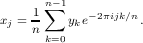
discrete Fourier transform — The (one-dimensional) discrete
Fourier transform (DFT) y0,…,yn-1 of a sequence of complex
numbers x0,…,xn-1 is given by the summation
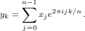 (The multi-dimensional generalization is straightforward). The xj are
given by the inverse DFT of the yk:
(The multi-dimensional generalization is straightforward). The xj are
given by the inverse DFT of the yk:
 (Frequently the forward and inverse transforms are defined in the
manner opposite to that given here, and the 1
n normalization
factor sometimes is moved about.) The DFT arises most
naturally in numerically approximating the Fourier coefficients
cm = 1 _
2π ∫
02πf(x)e-imxdx of a 2π-periodic function f which is
representable by the trigonometric series ∑
m=-∞∞cmeimx. The
fast Fourier transform algorithm (q.v.) can be used for efficient numerical
evaluation of the DFT.
(Frequently the forward and inverse transforms are defined in the
manner opposite to that given here, and the 1
n normalization
factor sometimes is moved about.) The DFT arises most
naturally in numerically approximating the Fourier coefficients
cm = 1 _
2π ∫
02πf(x)e-imxdx of a 2π-periodic function f which is
representable by the trigonometric series ∑
m=-∞∞cmeimx. The
fast Fourier transform algorithm (q.v.) can be used for efficient numerical
evaluation of the DFT.
disk hog — a derogatory term, used to connote a computer user
whose disk data files are excessively voluminous or numerous,
therefore putting other computer users at a relative disadvantage.
Unneeded data files should be scratched, or destroyed, in order to free
up disk space. Large disk files which will not be needed for a time
should be backed-up on magnetic tape and then deleted from
disk.
dynamic range — a summary measure of image quality
indicative of the ability to discern dim features when relatively
stronger features are present—i.e., a measure of the ability to
distinguish the dim features from artifacts of the image reconstruction
procedure (in a radio map, from remnants of the sidelobes of stronger
features) and from noise. The dynamic range achievable in a radio
interferometer map is determined primarily by the uniformity of the
u-v coverage, the density and extent of the coverage, the sensitivity of
the array, and the quality of the calibration.
If the true radio source brightness distribution f is known, one can
define the dynamic range of a reconstruction  as, say, the ratio of
the maximum value of |f| to the r.m.s. difference between f
and
as, say, the ratio of
the maximum value of |f| to the r.m.s. difference between f
and  . When f is unknown, as is usually the case, an empirical
measure of the dynamic range is used—perhaps the ratio of the
maximum value of |
. When f is unknown, as is usually the case, an empirical
measure of the dynamic range is used—perhaps the ratio of the
maximum value of | | to the r.m.s. level in an apparently empty
region of the map, or the ratio of the strongest feature to the
weakest “believable” feature—, but there is no widely-accepted
definition.
| to the r.m.s. level in an apparently empty
region of the map, or the ratio of the strongest feature to the
weakest “believable” feature—, but there is no widely-accepted
definition.
What one might wish to call the “true” dynamic range of a radio
map is a spatially-variant quantity. The ability to discern a dim feature
depends on its proximity to brighter features, because there are
relatively stronger sidelobe remnants near the bright features. The
quality of a map (and perhaps the dynamic range—depending on how
it is defined) deteriorates away from the phase tracking center, because
of the inability of the image reconstruction algorithms to compensate
for various instrumental effects (e.g., bad pointing, bandwidth smearing,
etc.).
EDT — a sophisticated text editor (a screen editor) used on
the Vaxes. It makes use of the “keypad” feature of the fancier
terminals. EDT can be run only on certain model terminals: on the
DEC (Digital Equipment Corp.) Models VT–52 and VT–100,
and on terminals such as the Visual–50’s and the Visual–100’s
which are capable of emulating the DEC terminals. See text
editor.
EMACS — a sophisticated text editor used on the Vaxes, as well
as on many computers which run under the UNIX operating system.
(There is also a version for the IBM-PC.) EMACS is a screen editor,
and the one which is favored by most among those in the AIPS
programming group. On terminals with the “keypad” feature, the
keypad keys can be programmed by the user to perform many
useful editing tasks; however, EMACS can be run from other
models of terminals, as well. EMACS provides two powerful and
convenient features which most other text editors do not offer:
the ability to temporarily exit from the editor and “return to
monitor level,” and the ability to initiate an interactive “job
control session,” or initiate sub-tasks, in an EMACS buffer. See text
editor.
explain file — in AIPS, a text file containing a detailed
explanation of a particular AIPS task or verb, often including hints,
suggested applications, algorithmic details, and bibliographical
references. Issuing the AIPS verb EXPLAIN causes the contents of an
explain file to be printed on the terminal screen or on a line printer.
Compare help file.
EXPORT format — a visibility data magnetic tape format for
transport of VLA data from the DEC–10 computer or the on-line
computer at the VLA.
EXPORT tape — a magnetic tape containing data recorded in
the EXPORT format.
exp × sinc function — a useful gridding convolution function:
same as the Gaussian-tapered sinc function (q.v.), except that the exponent of the argument to the exponential function may be other
than two.
extension file — in AIPS, a data file containing data supplemental
to those contained in a primary data file (either a u-v data file or an image
file). Whenever a primary data file is deleted by the standard
mechanism within AIPS for file destruction, all extension files
associated with that primary data file also are destroyed. Extension
files, however, may be deleted without deleting the the associated
primary data file.
Extension files are grouped into categories of named types.
Examples: plot files, history files, slice files, gain files, etc.
When an AIPS task creates a new primary data file from an old
one, generally it attaches, to the new file, clones of any extension
files associated with the old file that remain relevant to the new
one.
false color display — In digital imagery, a false color display is
one which is generated by using a number n > 1 of real-valued
functions f1(x,y),…,fn(x,y) to control the proportions, at each
pixel coordinate (x,y), of an additive mixture of three primary
hues. In practical terms, the user of a digital display system
supplies f1,…,fn, and twists knobs that control the mapping
Rn → R3 that sends the n pixel values at each (x,y) into the
proper image chromaticity and intensity. Compare pseudo-color
display.
A so-called true color display is obtained with n = 3 and with
transfer functions chosen such that the color assignment corresponds in
an approximate way to the actual coloration of a scene (as in a color
photograph).
fast Fourier transform algorithm — a fast algorithm for the
computation of the discrete Fourier transform (DFT) y0,…,yn-1 of a
sequence of n complex numbers x0,…,xn-1,
 typically requiring only O(n log n) arithmetic operations — or a
multi-dimensional generalization thereof. By contrast, straightforward,
or naïve evaluation of the DFT requires O(n2) operations. The fast
Fourier transform algorithms (FFT’s) which currently are the most
popular are the Cooley–Tukey (1965) algorithms, for the case of n
highly composite. For n a power of two, the (radix-2) Cooley–Tukey
FFT requires about 2n log 2n real multiplications and 3n log 2n real
additions. More generally, the Cooley–Tukey algorithms require a
few times nσ(n) complex arithmetic operations, where σ(n) is
the sum of the prime factors of n, counting their multiplicities.
S. Winograd has produced FFT algorithms which are more
efficient than those of Cooley and Tukey, typically requiring
about the same number of additions, but only about 20% the
number of multiplications. (Computation of the required complex
exponentials—or sines and cosines—is not counted, since these
generally are either pre-computed and stored in compact tables, or
generated recursively.)
typically requiring only O(n log n) arithmetic operations — or a
multi-dimensional generalization thereof. By contrast, straightforward,
or naïve evaluation of the DFT requires O(n2) operations. The fast
Fourier transform algorithms (FFT’s) which currently are the most
popular are the Cooley–Tukey (1965) algorithms, for the case of n
highly composite. For n a power of two, the (radix-2) Cooley–Tukey
FFT requires about 2n log 2n real multiplications and 3n log 2n real
additions. More generally, the Cooley–Tukey algorithms require a
few times nσ(n) complex arithmetic operations, where σ(n) is
the sum of the prime factors of n, counting their multiplicities.
S. Winograd has produced FFT algorithms which are more
efficient than those of Cooley and Tukey, typically requiring
about the same number of additions, but only about 20% the
number of multiplications. (Computation of the required complex
exponentials—or sines and cosines—is not counted, since these
generally are either pre-computed and stored in compact tables, or
generated recursively.)
A further advantage of the FFT algorithms is their avoidance of
round-off error, which can build up severely when the DFT is evaluated
by brute-force. There are related, fast algorithms for the convolution of
sequences of real numbers, for the discrete cosine transform, etc.
Algorithmic details may be found in [H. J. Nussbaumer, Fast Fourier
Transform and Convolution Algorithms, Springer–Verlag, Berlin,
1982]. The computational complexity of the DFT is discussed by
L. Auslander and R. Tolimieri [Is computing with the finite
Fourier transform pure or applied mathematics, Bull. (New Series)
Amer. Math. Soc., 1 (1979) 847–897].
AIPS programs which use the FFT make use of the Cooley–Tukey
algorithm. When an array processor is used to compute the large
two-dimensional DFT’s of data which reside on disk, as typically is
required in synthesis mapping, the input/output time greatly exceeds
the actual computation time.
FFT — See fast Fourier transform algorithm.
FITS format — (Flexible Image Transport System) a magnetic
tape data format well-tailored for the transport of image data among
observatories. The FITS format is recommended for bringing
data into and out of AIPS. See [D. C. Wells, E. W. Greisen,
and R. H. Harten, FITS: A flexible image transport system,
Astron. Astrophys. Suppl. Ser., 44 (1981) 363–370]. Also see u-v FITS
format and FITS tape.
FITS tape — a magnetic tape containing data recorded in the
FITS format. FITS format data blocks are 2880 bytes in length. The
resultant tape blocking efficiency is 83%, 75%, and 61% at recording
densities of 800, 1600, and 6250 bpi, respectively.
flagging — in AIPS, the act of discarding one or more visibility
data points by setting a u-v data flag (q.v.). Compare clipping.
fringe rotator — in a correlating-type radio interferometer, a
mechanism to introduce a time-varying phase shift into the local
oscillator signal of a receiver, in order to reduce the frequency of the
oscillations of the correlator output. Fringe rotation allows the
correlator output (whose amplitude is proportional to visibility
amplitude) to be sampled at a lower rate. The natural fringe frequency
can be as high as 200 Hz on the VLA. The fringe rotation is chosen so
that the fringe frequency for a point source located at the so-called
fringe stopping center would be reduced to zero, or at least close to zero.
Usually the fringe stopping center and the delay tracking center
coincide; both then are called the visibility phase tracking center.
For further details, see A. R. Thompson’s Lecture No. 2 and
L. R. D’Addario’s Lecture No. 4 in the Third NRAO Synthesis Imaging
Summer School, and see R. M. Hjellming and J. Basart’s Ch. 2 of the
Green Book.
full-synthesis map — in earth-rotation aperture synthesis, with
stationary interferometer elements, a map derived from an observation
which is of such lengthy duration that the fullest possible u-v coverage
is obtained (i.e., from an observation extending from “horizon to
horizon”). Compare snapshot.
gain file — in AIPS, an extension file, associated with a u-v data file,
in which a table of approximate antenna/i.f. gains (typically obtained
by self-calibration) is stored.
Gaussian-tapered sinc function — A useful gridding
convolution function (q.v.), of support width equal to the width mΔu
of m u-v grid cells, is given by the separable product of two
Gaussian-tapered sinc functions, each of the form
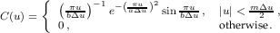 The choice m = 6, a ≃ 2.52, and b ≃ 1.55, yields what is, in a
certain natural sense, an optimal gridding convolution function of
this particular parametric form (see [F. R. Schwab, Optimal
gridding, VLA Scientific Memo. No. 132]). Also see spheroidal
function.
The choice m = 6, a ≃ 2.52, and b ≃ 1.55, yields what is, in a
certain natural sense, an optimal gridding convolution function of
this particular parametric form (see [F. R. Schwab, Optimal
gridding, VLA Scientific Memo. No. 132]). Also see spheroidal
function.
Gerchberg–Saxton algorithm — a simple iterative algorithm
which, in the field of signal processing, is used for the extrapolation of
band-limited signals—and, in image processing, for deconvolution. Assume that the Fourier transform  of an image f has been measured
over a region B, and that f is known to be confined to a region A. Let
χA denote the characteristic function of A and χB that of B. Denote the
measured data by ĝapprox—i.e., ĝapprox = χB
of an image f has been measured
over a region B, and that f is known to be confined to a region A. Let
χA denote the characteristic function of A and χB that of B. Denote the
measured data by ĝapprox—i.e., ĝapprox = χB + error. From the
initial approximant f0 (f0 ≡ 0 may be used) a sequence fn of
successive approximants to f is obtained, via the formula
+ error. From the
initial approximant f0 (f0 ≡ 0 may be used) a sequence fn of
successive approximants to f is obtained, via the formula
 Here, ˇ denotes inverse Fourier transform, and μ is a fixed
scalar, analogous to the loop gain parameter of the Högbom Clean
algorithm.
Here, ˇ denotes inverse Fourier transform, and μ is a fixed
scalar, analogous to the loop gain parameter of the Högbom Clean
algorithm.
To apply the algorithm in radio interferometry, one may identify
χB with the u-v sampling distribution and think of A to be analogous to
a Clean window. Denoting the dirty map by g and the dirty beam by b, the
iteration can be written as
 The Gerchberg–Saxton algorithm has been implemented by Tim
Cornwell in an AIPS program named APGS. APGS includes an ad hoc
non-negativity constraint—at each iteration, any pixel value which
would be driven negative is modified to become non-negative.
Convergence usually is sluggish.
The Gerchberg–Saxton algorithm has been implemented by Tim
Cornwell in an AIPS program named APGS. APGS includes an ad hoc
non-negativity constraint—at each iteration, any pixel value which
would be driven negative is modified to become non-negative.
Convergence usually is sluggish.
Some algorithms which are very similar to the Gerchberg–Saxton
algorithm are the Lent–Tuy algorithm, which is used in medical
imaging, the Papoulis, or Papoulis–Youla algorithm, used in signal
processing, and the so-called method of alternating orthogonal
projections, used in image reconstruction. See [J. L. C. Sanz and
T. S. Huang, Unified Hilbert space approach to iterative least-squares
linear signal restoration, J. Opt. Soc. Am., 73 (1983) 1455–1465] and
references cited therein.
Gibbs’ phenomenon — in the neighborhood of a discontinuity
of a periodic function f, the overshoot and oscillation (or ringing) of
the partial sums Sn of the Fourier series for f. In the vicinity of a
simple jump discontinuity, Sn always overshoots the mark by about
9%, regardless how large n. See [H. S. Carslaw, Introduction to the
Theory of Fourier’s Series and Integrals, Dover, New York, 1930,
ch. IX].
In harmonic analysis, often the Fourier coefficients are multiplied
by a weight function tending smoothly to zero at the boundaries of its
support, in order to smooth out the discontinuities and thereby reduce
the ringing in the synthesized spectrum. (This degrades the spectral
resolution, however.) See Hanning smoothing. For a discussion of
Gibbs’ phenomenon in the context of VLA cross correlation analysis,
see Larry D’Addario’s Lecture No. 4 in the Third NRAO Synthesis
Imaging Summer School.
GIPSY — (Groningen Image Processing System) a data
reduction system, similar in scope to AIPS, used in the Netherlands
for analysis of Westerbork Synthesis Radio Telescope (WSRT)
data.
global fringe fitting algorithm — an antenna-based algorithm
(in the spirit of the self-calibration algorithm) for VLBI fringe search. For
an n element array, the classical VLBI fringe fitting technique,
a correlator-based method, requires the estimation of n2 - n
parameters. The global fringe fitting method reduces this number to
3n - 3. Expressing the antenna/i.f. gain for antenna k of the array as
gk(t,ν) = akeiψk(t,ν) (here we include a frequency dependence) one
has that the observed visibility on the i–j baseline, to first-order, is
given by
where V ij is the true visibility, and where the rk are the antenna
residual fringe rates and the τk the antenna residual delays.
Given a source model, one may solve for the ψk(t0,ν0), the rk,
and the τk, using either a least-squares method or a Fourier transform
method. Because of the overdeterminacy provided by a simultaneous
solution for the parameters, this method allows proper delay
and fringe rate compensation of data on baselines of too low
signal-to-noise for the correlator-based method to work effectively. A
full description of the method is given in [F. R. Schwab and
W. D. Cotton, Global fringe search techniques for VLBI, Astron. J., 88
(1983) 688–694]. This algorithm is implemented in the AIPS program
CALIB.
graphics overlay plane — same as graphics plane.
graphics plane — a storage area within a TV display device, such
as the I2S, in which a full screen load of one-bit graphics information
(labeling, plotting, axis lines, etc.) is stored. A typical I2S unit is
equipped with four graphics planes, each 512 pixels × 512 pixels in
area. Compare image plane.
gray-scale display — a black-and-white display of a digitized
image—typically either a photographic or a video display.
gray-scale memory plane — same as image plane.
Green Book — An Introduction to the NRAO Very Large Array,
edited by R. M. Hjellming, NRAO, Socorro, NM—a useful reference
on many of the technical aspects of the VLA.
green screen — same as TEK screen.
gridding convolution function — in radio interferometer map
making, a function C—usually supported on a square the width of,
say, six u-v grid cells—with which the u-v measurement distribution is
convolved. The purpose is twofold: 1) to interpolate and smooth the
data, so that samples may be taken over the lattice points of a
rectangular grid (in order that the fast Fourier transform algorithm
may be applied) and 2) to reduce aliasing (the convolution in the u-v
plane induces a taper in the map plane). See aliased response,
gridding correction function, cell-averaging, dirty map, and uniform
weighting.
With judicious choice of C, a high degree of aliasing suppression is
possible. A high degree of suppression is desirable, even when there
are no “confusing” radio sources very near the field of interest,
because the effect is not only to reduce the spurious responses due to
sources lying outside of the field of view, but also to reduce the
response to sidelobes of the source of interest, which too are
aliased into the map from outside the field of view. See spheroidal
function.
gridding correction function — in radio interferometry, the
reciprocal 1∕Ĉ of the Fourier transform (FT) of the gridding convolution
function C. Since the map plane taper induced by the gridding
convolution usually is very severe, the dirty map normally is corrected
by point-wise division by the FT of the convolution function.
Obviously C should be chosen such that Ĉ has no zeros within the
region that is mapped. See dirty map.
gripe — in AIPS, an entry in the gripe file (q.v.).
gripe file — in AIPS, a disk file repository for formal reports of
program bugs, and for formal complaints and suggestions of a more
general nature. A mechanism by which the user may enter gripes
into the gripe file is activated by the issuance of the AIPS verb
GRIPE. The AIPS group provides prompt, written responses to all
gripes.
Hanning smoothing function — in the analysis of power
spectra, a weight function w by which the measured correlation
function is multiplied, in order to reduce that oscillation (Gibbs’
phenomenon) in the computed spectrum which is due to having
sampled at only a finite number of lags. w, as a function of lag, is given
by
 This is equivalent to convolving the discrete spectrum with the
sequence {
This is equivalent to convolving the discrete spectrum with the
sequence { ,
, ,
, }.
}.
Hanning smoothing sometimes is applied to the cross correlation
measurements obtained in VLA spectral line observing, in order to
reduce the effect of sharp bandpass filter cutoffs. It also is used
frequently in radio astronomical autocorrelation spectroscopy. See
Gibbs’ phenomenon, and for more on smoothing see [R. B. Blackman
and J. W. Tukey, The Measurement of Power Spectra, Dover, New York,
1958].
hard copy — computer output printed on paper (rather than, say,
written on magnetic tape); e.g., a printed contour plot or gray scale
display, or a listing of a catalog file.
hardware mount — the combined acts of installing a computer
external storage module, such as a disk pack or a reel of magnetic tape,
in some electro-mechanical unit (e.g., a disk drive or a tape drive) that
provides computer access to this data storage medium, and placing
that unit in readiness to be operated under computer control (e.g.,
positioning a magnetic tape at the BOT marker). Compare software
mount.
header record — a distinguished record within a data
file—generally the first record—which serves to define the contents of
the other records in the file by supplying relevant parameters, units of
measurement, etc.; also termed simply header.
In AIPS, however, the header record of each primary data file is
stored apart from that file, in a file which is termed a “CB” file. And a
directory, termed a catalog file (q.v.), or “CA” file, of all of each
user’s primary data files on a given disk is stored on that disk.
AIPS extension file headers are stored within the extension files
themselves.
help file — in AIPS, a text file, whose contents may be displayed on
the terminal screen of the interactive user, giving a brief explanation of
a particular AIPS verb, adverb, pseudo-verb, task, or miscellaneous
general feature. Compare explain file.
Hermitian function — a complex-valued function, of one or
more real variables, whose real part is an even function and whose
imaginary part is odd. The Fourier transform (FT) of a real-valued
function is Hermitian, and the inverse FT of a Hermitian function is
real.
Since each of the radio brightness distributions I(x,y),
Q(x,y), U(x,y), and V (x,y) representing Stokes’ parameters is
real-valued, Stokes’ visibility functions have the property of conjugate
symmetry: V I(-u,-v) = V I(u,v), V Q(-u,-v) = V Q(u,v),
V U(-u,-v) = V U(u,v), and V V (-u,-v) = V V (u,v). (Here,
V I = Î, V Q =  , etc., where ˆ denotes FT.)
history file — in AIPS, an extension file containing a summary of
all, or most of the processing, by AIPS tasks, of the data recorded in all
associated files.
Hogbom Clean algorithm — a deconvolution algorithm
devised by Jan Högbom for use in radio interferometry [J. A.
Högbom, Aperture synthesis with a non-regular distribution of
interferometer baselines, Astron. Astrophys. Suppl. Ser., 15 (1974)
417–426]. Denote (the discrete representations of) the dirty map by g
and the dirty beam by b. The algorithm iteratively constructs
discrete approximants fn to a solution f of the equation b * f = g,
starting with an initial approximant f0 ≡ 0. At the nth iteration,
one searches for the peak in the residual map g - b * fn-1. A
δ-function component, centered at the location of the largest residual,
and of amplitude μ (the loop gain) times the largest residual, is
added to fn-1 to yield fn. The search over the residual map is
restricted to a region A termed the Clean window. The iteration
terminates with an approximate solution fN either when N
equals some iteration limit Nmax, or when the peak residual (in
absolute value) or the r.m.s. residual decreases to some given
level.
To diminish any spurious high spatial frequency features in the
solution, fN is convolved with a narrow elliptical Gaussian function
h, termed the Clean beam. Generally h is chosen by fitting to the central
lobe of the dirty beam. Also, one generally adds the final residual map
g - b * fN to the approximate solution fN * h, in order to produce a
final result, termed the Clean map, with a realistic-appearing level of
noise. See super-resolution.
host computer — In the parasitic relationship of a computer
program or program package, such as AIPS, to the computer on
which it runs, the latter is termed the host computer. Also, in the
master–slave relationship of a computer to one of its peripheral
devices, such as an array processor, the master may be termed the
host.
hue — one of the three basic parameters (hue, intensity, and
saturation) which may be used to describe the physical perception of
the light that reaches one’s eye. Hue, which is also termed tint, or
simply color, refers to the dominant wavelength of the coloration, at a
given location in an image or scene. The term also may be used to
describe a multi-modal color spectrum—e.g., one speaks of a
purple hue. Different spectral distributions of light, of identical
intensity and saturation, are capable of producing identical retinal
responses; these unique responses comprise the set of perceptible
hues.
Color matching tests have established that there are three basic
types of human retinal receptors, whose peak responses are to
red, green, and blue light. These are the three primary hues used
in additive color mixing—e.g., in digital image display. They
may be used to produce all, or virtually all, of the perceptible
hues.
See C.I.E. chromaticity diagram.
hybrid mapping algorithm — an algorithm for calibration of
radio interferometer data which is essentially equivalent to the
self-calibration algorithm (q.v.) (used in VLA data reduction), except in
that it makes explicit use of the closure phase and closure amplitude
relations, rather than explicit use of the relation Ṽij = gigjV ij relating
observed visibility to the product of the true visibility and a pair of
antenna/i.f. gains. Hybrid mapping, which is used extensively in VLBI
data reduction, is described in [A. C. S. Readhead et al., Mapping
radio sources with uncalibrated visibility data, Nature, 285 (1980)
137–140].
Either algorithm (assuming that one cares to make some
distinction) can be applied to data obtained with connected- (e.g., the
VLA) and non-connected-element interferometers (e.g., VLBI arrays).
Any differences in the results produced by the two algorithms would
be attributable primarily to differences in the effective weighting of the
data (in particular, early implementations of both algorithms
discarded data which could have been used to obtain over-determined
solutions for the calibration parameters).
IIS — See I2S.
image — in the context of AIPS, any finite-volume, linear,
rectangular, or hyper-rectangular array of pixels; e.g., a digitized
photograph, or a radio map. The term also is used (less technically) to
refer to the display of data—e.g., a television picture of a radio
map.
image catalog — in AIPS, a disk file containing data records
describing the data stored on the TV display device image planes. These
records are essentially identical in structure to the header records stored
in the catalog file. The data in the image catalog furnish the information
that is required for proper axis labeling, pixel value retrieval,
etc.
image file — in AIPS, a primary data file whose content is an
image.
image plane — a storage area within a TV display device, such
as the I2S, in which a full screen load of single word pixels is stored.
A typical I2S unit is equipped with four image planes, each
512 pixels × 512 pixels in area (each pixel is represented by eight bits).
Often several image planes are used at one time—either for
black-and-white or pseudo-color display of a large image, sections of
which may occupy different image planes—or for false color or true
color display of a smaller image, now using, say, three image
planes—one to control each of the three electron guns (for red,
green, or blue phosphor) in the TV display. Compare graphics
plane.
image reconstruction — the attempted recovery of an
image after it has undergone the distorting effects, the blurring,
etc., produced by some physical measurement and recording
device, such as a camera, a radio interferometer, or a tomography
machine. The operation of many measurement devices can be
adequately modeled by a linear Fredholm integral equation of the first
kind. In the two-dimensional case, e.g., one assumes that the
measurement g(x,y) is related to the undistorted image f(x,y) by the
equation
 (Often it is convenient to use the more compact, operator notation,
g = Kf + ϵ.) The kernel K of the equation is called the point spread
function, (q.v.). Measurement error and the error arising from any
simplifying assumptions are lumped together into the ϵ(x,y)
term. Some particularly well-behaved measurement systems can
be adequately modeled by a simple convolution equation, in
which case K is given by K(x,y,x′,y′) = h(x - x′,y - y′).
This is the case, e.g., when the VLA is used to observe a small
‘unconfused’ radio source; then g may be identified with the
dirty map and h with the dirty beam. Or when K, considered as a
function of (x,y), is given at each (x′,y′) by the delay beam for that
position, the equation models the bandwidth smearing effect (q.v.);
as the bandwidth → 0, the convolution model again becomes
valid.
(Often it is convenient to use the more compact, operator notation,
g = Kf + ϵ.) The kernel K of the equation is called the point spread
function, (q.v.). Measurement error and the error arising from any
simplifying assumptions are lumped together into the ϵ(x,y)
term. Some particularly well-behaved measurement systems can
be adequately modeled by a simple convolution equation, in
which case K is given by K(x,y,x′,y′) = h(x - x′,y - y′).
This is the case, e.g., when the VLA is used to observe a small
‘unconfused’ radio source; then g may be identified with the
dirty map and h with the dirty beam. Or when K, considered as a
function of (x,y), is given at each (x′,y′) by the delay beam for that
position, the equation models the bandwidth smearing effect (q.v.);
as the bandwidth → 0, the convolution model again becomes
valid.
Except in trivial cases, solution of the Fredholm equation always is
an ill-posed problem. Mild conditions on K and f (the classical ‘Picard
conditions’—see F. Smithies [Integral Equations, Cambridge Univ. Pr.,
London, 1958]) ensure the existence of (non-unique) solutions
when ϵ ≡ 0. But, because of the effect of measurement noise, one
usually does not seek an exact solution, but rather an approximate
solution—one which fits the data to within the measurement errors.
Uniqueness and regularity of the computed approximate solution
are obtained by imposing such constraints as known support,
non-negativity, and smoothness conditions. See regularization
method. Also see H. C. Andrews and B. R. Hunt [Digital Image
Restoration, Prentice–Hall, Englewood Cliffs, NJ, 1977] and phaseless
reconstruction.
inputs file — in AIPS, a text file, whose contents may be
displayed on the terminal screen of the interactive user, giving a
summary of the adverbs relevant to a given verb or a given AIPS
task.
instrumental polarization — any contamination of a
polarization measurement by an instrument’s response to an
undesired polarization state. In radio interferometry, the instrumental
polarization arises mainly from feed imperfections and from
plumbing leaks between the feeds and the receiver front-ends. One
tries to remove the instrumental polarization by applying corrections
derived from observations of calibration sources whose polarization
properties are known. Within AIPS, there is, at present, no facility for
polarization calibration. The polarization calibration of VLA data
normally takes place on the DEC–10 computer at the VLA. For more
details, see Carl Bignell’s Lecture No. 4 in the 1985 Summer School
Proceedings. See beam squint.
intensity — one of the three basic parameters (hue, intensity, and
saturation) which may be used to describe the physical perception of
color. Intensity is a measure of the energy of the spectral distribution,
at a given point in an image or scene, weighted by the spectral
response of the visual system. Luminance is the energy of the physical
spectrum, but not weighted by the visual response. Brightness
sometimes is used synonymously with either term.
See C.I.E. chromaticity diagram.
invisible distribution — in the context of radio interferometry,
a function f (or a generalized function—or distribution) whose
Fourier transform  vanishes everywhere that the interferometer pairs
have sampled. This term was introduced by R. N. Bracewell and
J. A. Roberts [Aerial smoothing in radio astronomy, Austr. J. Phys., 7
(1954) 615–640]. Also see principal solution.
vanishes everywhere that the interferometer pairs
have sampled. This term was introduced by R. N. Bracewell and
J. A. Roberts [Aerial smoothing in radio astronomy, Austr. J. Phys., 7
(1954) 615–640]. Also see principal solution.
For an actual interferometer, there exist fewer physically plausible
invisible distributions than for an idealized interferometer. This is
because each visibility sample is not a point sample of  , but rather some kind of local average. By the Paley–Wiener theorem, if
  is
nontrivial and vanishes in some open neighborhood, then f
cannot be of compact support, and hence it may be considered
implausible.
is
nontrivial and vanishes in some open neighborhood, then f
cannot be of compact support, and hence it may be considered
implausible.
IPL — (Initial Program Load) same as boot.
isoplanaticity assumption — in the context of radio
interferometry (the term is used too in optics), the assumption that
over each element of an array all wavefronts arriving from different
parts of the sky to which the interferometer pairs are sensitive are
subject to identical atmospheric phase perturbations. A patch of sky
over which the assumption is valid is referred to as an isoplanatic
patch.
Approximate validity of the isoplanaticity assumption is a
necessary condition for the success of calibration (self-calibration, in
particular) of radio interferometer data (from an earth-based array) if
one is to rely on a model incorporating time-varying antenna/i.f. gains,
one per antenna, whose arguments (or phases) are to include the
atmospheric phase corruption. However, see F. R. Schwab [Relaxing
the isoplanatism assumption in self-calibration; applications to
low-frequency radio interferometry, Astron. J., 89 (1984) 1076–1081].
I2S — (International Imaging Systems Models 70 and 75) a TV
display device, capable of both black-and-white and color display,
manufactured by the Stanford Technology Corporation. At an
AIPS site typically it is equipped with four 512 pixel × 512 pixel
eight-bit image planes, four one-bit graphics planes, a trackball, and
sometimes an ALU. The eight-bit pixel representation (in the image
planes) allows the intensity of each of the three electron gun
beams to be set at any of 256 discrete levels. (Actually, 1024
levels can be used, because of an extra two bits of capability
provided in the transfer function tables and the internal arithmetic
unit.) An I2S is attached to three of the NRAO’s computers
on which the AIPS system runs (the VLA and Charlottesville
Vaxes).
line editor — a text editor (q.v.) which allows the modification of
single lines or records within a text file, but one which does not allow
the simultaneous modification of more than one line. SOS and SEDIT
are both line editors. Screen editors (q.v.) are more versatile than line
editors.
lobe rotator — same as fringe rotator, (q.v.).
loop gain — in the Högbom Clean algorithm, the fraction μ of
the largest residual which is used in determining the amplitude, or
flux, of a Clean component. Convergence can be achieved for μ in the
range (0, 2), but generally a small value, say μ = 1 _
10 , is recommended,
especially in dealing with extended sources. See Högbom Clean
algorithm.
luminance — See intensity.
l1 solution algorithm — See self-calibration gain solution
algorithm.
l2 solution algorithm — See self-calibration gain solution
algorithm.
major cycle — In the Clark Clean algorithm (q.v.), a number of
minor cycles, or inner iterations, followed by the computation by
the FFT algorithm of the full residual map, comprise a major
cycle.
map — an image, one or more of whose coordinate axes represents
some spatial coordinate.
maximum entropy method — a regularization method (q.v.) for
the numerical solution of ill-posed problems, given noisy data, in
which the regularizing (or smoothing) term—which measures the
roughness of the computed approximate solution  —is given
by the negative of the Shannon entropy of
—is given
by the negative of the Shannon entropy of  , -H(
, -H( ) : in the
continuous case, letting A denote the domain of definition of
) : in the
continuous case, letting A denote the domain of definition of  ,
H(
,
H( ) ≡-∫
A
) ≡-∫
A (x) log
  (x) dx, where
  has been normalized so
that ∫
A
has been normalized so
that ∫
A (x) dx = 1 (and 0 log 0 ≡ 0); and in the discrete case,
H(
(x) dx = 1 (and 0 log 0 ≡ 0); and in the discrete case,
H( ) ≡-∑
) ≡-∑ (xi) log
  (xi), where
  has been normalized so
that ∑
has been normalized so
that ∑ (xi) = 1. The underlying philosophy of the method,
espoused early on by Jaynes (“Jaynes’ method of prior estimation”,
[E. T. Jaynes, Prior probabilities, IEEE Trans. Syst. Sci. Cyb., SSC-4
(1968) 227–241]) and by J. P. Burg at a 1967 meeting of the Society
of Exploration Geophysicists, is that one is being “maximally
noncommittal” in regard to the insufficiency of the data if one
maximizes the entropy, and thus minimizes the “information content”,
of
(xi) = 1. The underlying philosophy of the method,
espoused early on by Jaynes (“Jaynes’ method of prior estimation”,
[E. T. Jaynes, Prior probabilities, IEEE Trans. Syst. Sci. Cyb., SSC-4
(1968) 227–241]) and by J. P. Burg at a 1967 meeting of the Society
of Exploration Geophysicists, is that one is being “maximally
noncommittal” in regard to the insufficiency of the data if one
maximizes the entropy, and thus minimizes the “information content”,
of  , subject to the constraint that
  should agree with the given
data.
should agree with the given
data.
For one-dimensional discrete convolution equations, with noiseless,
regularly-spaced data, there exists a closed-form solution—for other
cases, iterative methods are used, as with other forms of the
regularization method.
Use of the method in radio astronomy was encouraged by
J. G. Ables in 1972 in public lectures, and it now is in common
use in radio interferometry (cf. [S. F. Gull and G. J. Daniell,
Image reconstruction from incomplete and noisy data, Nature, 272
(1978) 686–690]). Non-negativity of the computed solution is a
natural by-product of the method. For reconstruction of polarized
brightness distributions in interferometry (Stokes’ Q, U, and V ),
which, unlike the total intensity, may assume negative values,
Ponsonby has derived an appropriate generalization of the method
[J. E. B. Ponsonby, An entropy measure for partially polarized
radiation…, Mon. Not. R. Astr. Soc., 163 (1973) 369–380]. See
Variational Method.
memory page — See virtual memory page.
memory paging — same as virtual memory page swapping.
memory thrashing — an excessive amount of virtual memory
page swapping (q.v.) on a computer (such as the Vax) with a virtual
memory operating system. A condition of memory thrashing is
likely to occur whenever too many programs with large memory
requirements are active (a single program with excessive memory
requirements also can cause memory thrashing).
message file — in AIPS, a text file containing progress report
messages generated during the execution of AIPS tasks and also
containing a chronicle of the user’s interaction (via verb commands)
with AIPS. Each AIPS user is assigned a message file, the contents of
which may be printed out, typed upon a terminal display screen, or
emptied—at will—by invoking the appropriate verb command. See
AIPS monitor.
message terminal — same as AIPS monitor.
minor cycle — in the Clark Clean algorithm (q.v.), an inner
iteration, in which the peak residual over a sub-region (the Clean
window) of the full residual map is found and is used to obtain the next
successive iterate. Compare major cycle.
microcode — See array processor microcode.
monitor — See AIPS monitor or Conrac monitor.
m × n map — The convention adopted for AIPS is opposite the
standard matrix algebra terminology: whereas an m × n matrix is
comprised of m rows and n columns, an m × n map or image in AIPS
has, in the usual display format, m pixels along the horizontal axis
(usually termed the x-axis) and n pixels along the vertical axis
(usually termed the y-axis). Moreover, pixels of a two-dimensional
map in the usual display format are numbered from the bottom
left-hand corner: the pixel location specified by the ordered pair (i,j)
is in column number i and row number j, counting from the bottom
left. In other than two-dimensional “images”, the (1,…, 1) pixel is
also said to be at the “bottom left corner” (BLC), just as in the
two-dimensional case. See data cube, pixel coordinates, and coordinate
reference pixel.
MX — See “battery-powered” Clean algorithm.
natural weighting — See uniform weighting.
negative bowl artifact — See zero-spacing flux.
non-closing offset — See correlator offset.
Nyquist sampling rate — the slowest rate of sampling which,
according to the Shannon sampling theorem (q.v.), would allow a
band-limited function f(t) to be recovered via the Shannon series. If the
smallest symmetric interval which contains the support of the Fourier
transform of f is the interval [-a,a], then the Nyquist sampling rate
for f is 2a; i.e., the interval between samples (the sampling period)
must be less than the reciprocal bandwidth 1∕2a. The terms
oversampling and undersampling refer to sampling at rates faster or
slower than the Nyquist rate. The difference between f and the
Shannon series formed from too coarsely spaced samples is called
aliasing.
operating system —
page — See virtual memory page and terminal page.
page swapping — See virtual memory page swapping.
Paley–Wiener theorem — The classical Paley–Wiener theorem
says that a square-integrable complex-valued function  , defined over
the real line, can be extended off the real line as an entire function of
exponential type ≤ 2πa if and only if f(x) ≡ 0 for |x| > a —i.e., iff
, defined over
the real line, can be extended off the real line as an entire function of
exponential type ≤ 2πa if and only if f(x) ≡ 0 for |x| > a —i.e., iff  is band-limited to [-a,a] (here ˆ denotes Fourier transform). (An
everywhere-analytic function g(z) is said to be of exponential type
≤ A if ∃c such that, for all z, |g(z)|≤ ceA|z|.) For a derivation, see
H. Dym and H. P. McKean [Fourier Series and Integrals, Academic
Press, 1972]. The Shannon series is a means of extending
is band-limited to [-a,a] (here ˆ denotes Fourier transform). (An
everywhere-analytic function g(z) is said to be of exponential type
≤ A if ∃c such that, for all z, |g(z)|≤ ceA|z|.) For a derivation, see
H. Dym and H. P. McKean [Fourier Series and Integrals, Academic
Press, 1972]. The Shannon series is a means of extending  to
C. The extension of the Paley–Wiener theorem to the case of
generalized functions (to tempered distributions) is called the
Paley–Wiener–Schwartz theorem.
to
C. The extension of the Paley–Wiener theorem to the case of
generalized functions (to tempered distributions) is called the
Paley–Wiener–Schwartz theorem.
The Fourier transform  : Rn → C of a function f with
support in a given n-dimensional convex compact set K can
be analytically extended to all of Cn. Growth properties on
: Rn → C of a function f with
support in a given n-dimensional convex compact set K can
be analytically extended to all of Cn. Growth properties on  which are sufficient in order for the converse to hold are given by
K. T. Smith, D. C. Solomon, and S. L. Wagner [Practical and
mathematical aspects of the problem of reconstructing objects
from radiographs, Bull. Amer. Math. Soc., 83 (1977) 1227–1270]
(in addition to the classical version of the multi-dimensional
Paley–Wiener theorem, for rectangular K, they give versions with
tighter growth bounds, and for arbitrary convex K). Smith et al. use
the Paley–Wiener theorems to establish indeterminacy theorems for
tomographic reconstruction. Their results are also relevant to Fourier
synthesis, because of the connection between the two-dimensional
Fourier transform and the one-dimensional Radon transform. The
Paley–Wiener theorems have also been used in establishing
results on the problem of phaseless reconstruction (q.v.) and in
proving the convergence of constrained Gerchberg–Saxton-type
algorithms (see A. Lent and H. Tuy [An iterative method for the
extrapolation of band-limited functions, J. Math. Anal. Appl., 83
(1981) 554–565]).
which are sufficient in order for the converse to hold are given by
K. T. Smith, D. C. Solomon, and S. L. Wagner [Practical and
mathematical aspects of the problem of reconstructing objects
from radiographs, Bull. Amer. Math. Soc., 83 (1977) 1227–1270]
(in addition to the classical version of the multi-dimensional
Paley–Wiener theorem, for rectangular K, they give versions with
tighter growth bounds, and for arbitrary convex K). Smith et al. use
the Paley–Wiener theorems to establish indeterminacy theorems for
tomographic reconstruction. Their results are also relevant to Fourier
synthesis, because of the connection between the two-dimensional
Fourier transform and the one-dimensional Radon transform. The
Paley–Wiener theorems have also been used in establishing
results on the problem of phaseless reconstruction (q.v.) and in
proving the convergence of constrained Gerchberg–Saxton-type
algorithms (see A. Lent and H. Tuy [An iterative method for the
extrapolation of band-limited functions, J. Math. Anal. Appl., 83
(1981) 554–565]).
phaseless reconstruction — the reconstruction of an image f
(see image reconstruction) from knowledge of (only) the magnitude | |
of the Fourier transform of f (and usually from only partial
knowledge of |
|
of the Fourier transform of f (and usually from only partial
knowledge of | |). Phaseless reconstruction has been considered for
the NRAO’s proposed millimeter wave interferometer array
[T. J. Cornwell, Imaging of weak sources with compact arrays, NRAO
Millimeter Array Memo. No. 12]. Recent results on phaseless
reconstruction appear in the JOSA Feature Issue on Signal Recovery
[J. Opt. Soc. Am., 73 No. 11 (Nov. 1983)]. Also see the papers by
J. R. Fienup and by R. H. T. Bates et al. in the 1983 Sydney Conference
Proceedings.
|). Phaseless reconstruction has been considered for
the NRAO’s proposed millimeter wave interferometer array
[T. J. Cornwell, Imaging of weak sources with compact arrays, NRAO
Millimeter Array Memo. No. 12]. Recent results on phaseless
reconstruction appear in the JOSA Feature Issue on Signal Recovery
[J. Opt. Soc. Am., 73 No. 11 (Nov. 1983)]. Also see the papers by
J. R. Fienup and by R. H. T. Bates et al. in the 1983 Sydney Conference
Proceedings.
phase tracking center — same as visibility phase tracking center,
(q.v.).
physical memory — core or semiconductor memory within a
computer (as opposed to slower memory—virtual memory, disk
storage, magnetic tape footage, etc.). A typical Vax is equipped with a
physical memory 3–4 megabytes in size.
pillbox — See cell-averaging.
pixel — (picture element) an element of a digitized image (or of a
map). A pixel is characterized by its position in the image and by its
numerical value. See m × n map, coordinate reference pixel, and pixel
coordinates.
pixel coordinates — in an AIPS image file, the pixels are
numbered consecutively, beginning with (1,…, 1) at the bottom left
corner (BLC) of the image. See coordinate reference pixel and m × n
map.
plot file — an AIPS extension file containing plotting information,
in the form of the commands which are necessary in order for a line
drawing peripheral device, such as a Calcomp or other pen plotter, a
green screen, or an electrostatic printer/plotter, to generate a
plot.
point source response — same as point spread function.
points per beam — in a digitized radio map, the characteristic
width, somehow defined, of the major lobe of the beam pattern, or
point spread function, divided by the pixel separation. Ordinarily the
number of points per beam is calculated by measuring the narrowest
diameter of the 50% contour level of the major lobe of the beam. To
avoid excessively severe discretization error, deconvolution
algorithms such as the Högbom Clean algorithm and the maximum
entropy method require, as a rule-of-thumb, at least three (and
preferably 4–5) points per beam.
point spread function — (PSF) 1. the response of a system or
an instrument to an impulsive, or point source, input. 2. in
radio interferometry, the response of the instrument to a point,
or unresolved, radio source—a fancy term for beam. Ignoring
instrumental effects, such as finite bandwidth and finite integration
time, the response does not depend upon the displacement of the
source away from the visibility phase tracking center—hence the term
space-invariant PSF (SIVPSF), and the contrary term space-variant PSF
(SVPSF).
A so-called linear space invariant measurement system (i.e., a
linear system with an SIVPSF) is equivalently described as a
system which can be modeled by a convolution equation; a linear
space-variant measurement system is modeled by a more general
linear Fredholm integral equation of the first kind. See image
reconstruction.
POPS — (People-Oriented Parsing System) the parser, or
command interpreter, embedded within the AIPS program; that part
of the AIPS program which attempts to interpret the user’s commands
(POPS symbols) and then initiate the appropriate reaction. POPS is
used in other astronomical data reduction programs at the NRAO: in
Condare, TPOWER/SPOWER, and the Tucson 12 m single-dish
packages.
POPS procedure — See POPS symbols.
POPS symbols — The AIPS user’s primary means of
communicating his wishes to AIPS is by typing commands, termed
POPS symbols, at the keyboard of a computer terminal. There are four
classes of POPS symbols: adverb, verb, pseudo-verb, and procedure. An
adverb is a symbol representing the storage area for a datum or for data
that are used to control the action of verbs, tasks, and procedures; that
is to say that the adverb symbols are used to set control parameters. A
verb is a symbol which causes POPS (or AIPS) to initiate some action
after POPS has finished interpreting, or compiling, the command line
typed at the computer terminal. A pseudo-verb is a symbol which
suspends, temporarily, the normal parsing of an input line and
which causes some action to take place while the line is being compiled, and, possibly, after compilation. A procedure is a symbol
representing a pre-compiled sequence of POPS symbols. Also see
task.
primary beam correction — in radio interferometry, the
multiplicative correction of a radio map by the reciprocal of an average
of the power patterns of the array elements. Measurements of the
primary beam parameters of the 25 m VLA elements are given by
Peter Napier and Arnold Rots in the memorandum [VLA primary
beam parameters, VLA Test Memo. No. 134, Feb. 1982]. There an
average power pattern and its reciprocal are approximated by
radial functions, polynomials in the distance from the pointing
position. The AIPS task PBCOR is used to apply this correction
to VLA maps. The appropriate correction at large distances
from the pointing position is not well-determined, thus PBCOR
“blanks” the map pixel values beyond a certain radius (see blanked
pixel).
primary data file — in AIPS, either a u-v data file, containing
measurements of the visibility function of a radio source, or an image
file, containing a digitized image or a radio map. Compare extension
file.
principal solution — in the context of radio interferometry, the
inverse Fourier transform of the u-v measurement distribution;
i.e., the dirty map (q.v.) in sense 1 of the definition. This term
was introduced by R. N. Bracewell and J. A. Roberts [Aerial
smoothing in radio astronomy, Austr. J. Phys., 7 (1954) 615–640].
Except in the trivial case, the principal solution to the mapping
problem in interferometry is a physically implausible solution,
because the principal solution has not the property of compact
support.
An invisible distribution (q.v.) added to the principal solution yields
another solution—i.e., another brightness distribution which is
consistent with the observations.
procedure — See POPS symbols.
prolate spheroidal wave function — an eigenfunction of
the finite, or truncated, Fourier transform—more precisely, for
given c, one of the countably many solutions of the integral
equation
 equivalently, a solution of the differential equation
(1 - η2)f′′- 2ηf′ + (b - c2η2)f = 0; or, equivalently, a solution of
the wave equation in a system of prolate spheroidal coordinates. The
eigenfunction of the above equation associated with the largest
eigenvalue ν is termed the 0-order solution.
equivalently, a solution of the differential equation
(1 - η2)f′′- 2ηf′ + (b - c2η2)f = 0; or, equivalently, a solution of
the wave equation in a system of prolate spheroidal coordinates. The
eigenfunction of the above equation associated with the largest
eigenvalue ν is termed the 0-order solution.
If we want a gridding convolution function C, of support width
equal to the width of m grid cells, that is optimal in the sense that its
Fourier transform Ĉ has the property that the concentration
ratio
 is
maximized, then C is the separable product of two 0-order prolate
spheroidal wave functions, with c = πm∕2. See gridding convolution
function and spheroidal function.
is
maximized, then C is the separable product of two 0-order prolate
spheroidal wave functions, with c = πm∕2. See gridding convolution
function and spheroidal function.
prompt character — a character (often the dollar sign “$” or the
greater-than sign “>”) which the computer program or the operating
system prints on the terminal screen of the interactive user in order to
prompt, or invite, a typed response from the user. The AIPS program’s
standard prompt character is the greater-than sign, and on the Vaxes at
the NRAO the operating system’s prompt character is the dollar sign.
On most UNIX systems, the prompt character is the percent
sign. Thus, most commands (or POPS symbols) peculiar to AIPS
must be typed on a line beginning with the >-character, and any
command to the operating system, such as the command to
mount a tape, must be typed on a line beginning with the $- or
%-character.
When operating in some lesser-used, special modes, AIPS employs
other prompt characters: “:” for procedure building, “;” for procedure
editing, “!” for entry of gripes, “<” for batch file preparation, and “#”
for parameter reading.
Prussian helmet Clean algorithm — a modified version of the
Högbom Clean algorithm, devised by Tim Cornwell. The idea is to
drive the Clean algorithm toward an approximate solution f of
minimal Euclidean norm—i.e., to find an f consistent with the data,
confined to the Clean window, comprised of a small number of
point components, and such that ∫
∫
Clean
window [f(x,y)]2 dxdy
is minimized. This is accomplished by adding a δ-function of
amplitude ω, centered at the origin, to the dirty beam, and then just
proceeding as normal with the Clean algorithm. Proper choice
of ω depends on the distribution of measurement errors. See
[T. J. Cornwell, A method of stabilizing the Clean algorithm,
Astron. Astrophys., 121 (1983) 281–285]. A provision for this
modification is incorporated in the AIPS tasks APCLN and MX. See
regularization method.
pseudo-AP — See pseudo-array processor.
pseudo-array processor — in AIPS, the term which is applied
to a collection of Fortran subroutines which may be used to emulate
the operation of an FPS Model AP–120B array processor. At
those AIPS sites which do not have an array processor, the AIPS
tasks which normally would make use of an array processor
use the pseudo-array processor subroutines instead. See array
processor.
pseudo-color display — In digital imagery, a pseudo-color
display is one which is derived from a single real-valued function
f(x,y) and a mapping R1 → R3 that controls the hue, intensity,
and saturation—or, equivalently, the proportions in an additive
mixture of three primary hues—of the coloration at each pixel
coordinate (x,y) of the display, according to the value of f(x,y). A
pseudo-color display might be used, for example, to represent
measurements of the intensity of the radio continuum flux density of a
source.
Compare false color display and see color contour display.
pseudo-continuum u-v data file — in VLA spectral line data
reduction, a u-v data file containing the visibility measurements from a
small number of spectral line channels, recorded in the same format as
continuum visibility data. The purpose is to enable the use, for
spectral line data analysis, of programs originally intended only to
handle continuum data reduction.
pseudo-verb — See POPS symbols.
PSF — See point spread function.
Q-routine — in AIPS, a primitive level subroutine designed to
function on a particular manufacturer’s production model of an array
processor. A goal of the AIPS project is to construct libraries of
Q-routines—one library appropriate to each model of array processor
which might be used in conjunction with AIPS—with identical names,
argument lists, and functionality. Existing Q-routines emulate the
standard library of Floating Point Systems, Inc.’s, model AP–120B
array processor.
quick boot — an abbreviated boot procedure. See boot.
RANCID — (Real (or Radio) Astronomical Numerical
Computation and Imaging Device) the name by which the AIPS data
reduction system formerly was known.
re-boot — Having booted once already, one re-boots. See
boot.
regularization method — in the numerical solution of ill-posed
problems, given noisy data, a method in which the original problem is
converted into a well-posed problem by requiring of the solution to
the modified problem (which now is an approximate solution to the
original problem) that it satisfy some smoothness constraint. The
prototypical ill-posed problem has the form Kf = g + ϵ, where K is a
known linear integral operator (e.g., a convolution operator), where
g + ϵ, which is given, represents some noisy measurement, and
where f is unknown. In the context of radio interferometry, one
may take g + ϵ to be the dirty map and K to be the operator
which convolves the “true” radio source brightness distribution f
with the dirty beam. Now, denoting our approximate solution
to the ill-posed problem by  ,
,  is found by minimizing the
expression
is found by minimizing the
expression
 for
some given choice of the regularization parameter λ, 0 < λ < 1.
∥g - K
for
some given choice of the regularization parameter λ, 0 < λ < 1.
∥g - K ∥2 is the mean squared residual (occasionally some other
measurement of the error is used), and S(
∥2 is the mean squared residual (occasionally some other
measurement of the error is used), and S( ) is a measure of the
roughness of the computed solution—say, some power of a norm or
seminorm of
) is a measure of the
roughness of the computed solution—say, some power of a norm or
seminorm of  , or a similar quantity, such as the negative of the
(Shannon) entropy of
, or a similar quantity, such as the negative of the
(Shannon) entropy of  .
.
Proper choice of λ must be based on statistical considerations
which depend on the distribution of measurement errors; often, one
chooses λ in order achieve an a priori reasonable value of the mean
squared residual. The maximum entropy method, Tikhonov regularization,
and the Prussian helmet Clean algorithm are special cases of the
regularization method. Appropriate choice of S is discussed
by J. Cullum [The effective choice of the smoothing norm in
regularization, Math. Comp., 33 (1979) 149–170], and the choice of S
and λ, by a statistical method known as “cross validation”, is
described by G. Wahba [Practical approximate solutions to linear
operator equations when the data are noisy, SIAM J. Numer. Anal.,
14 (1977) 651–677]. Often, some Sobolev norm is chosen for
S.
Usually, in addition to the smoothness constraint, f is assumed
to be of known, compact support. Other constraints, such as
non-negativity, may be included as well. In the case in which the data
are exact—i.e., when ϵ = 0, so that g = Kf—one may obtain
the regularized solution corresponding to λ = 0 as the limit
of regularized solutions  λ as λ → 0. See Variational Method.
Also see D. M. Titterington [General structure of regularization
procedures in image reconstruction, Astron. Astrophys., 144 (1985)
381–387].
λ as λ → 0. See Variational Method.
Also see D. M. Titterington [General structure of regularization
procedures in image reconstruction, Astron. Astrophys., 144 (1985)
381–387].
regularization parameter — in the regularization method
(q.v.) for the solution of ill-posed problems, a smoothing parameter λ,
0 < λ < 1, which controls the trade-off between an error term,
measuring agreement of the computed solution  with the given data,
and a term S(
with the given data,
and a term S( ), which measures the roughness of
  . I.e., λ controls
the amount of “regularization”. See super-resolution.
. I.e., λ controls
the amount of “regularization”. See super-resolution.
re-IPL — same as re-boot.
residual delay — Expressing the antenna/i.f. phase, ψk, for
antenna k of a VLBI array as a function of frequency as well as of time,
the residual delay on the i–j baseline at (t0,ν0) is given by
τij ≡ (t0,ν0), where ϕij denotes the visibility phase
on the i–j baseline. (The partial w.r.t. t is called the residual fringe rate.)
Usually the major contributor to residual delay is the difference in
the station clock errors. The residual delay is a group delay,
rather than a phase delay. It is termed residual because it is
assumed that geometric effects have already been compensated
for.
(t0,ν0), where ϕij denotes the visibility phase
on the i–j baseline. (The partial w.r.t. t is called the residual fringe rate.)
Usually the major contributor to residual delay is the difference in
the station clock errors. The residual delay is a group delay,
rather than a phase delay. It is termed residual because it is
assumed that geometric effects have already been compensated
for.
The “antenna components” of τij, namely τk ≡ (t0,ν0), are
called the antenna residual delays. They are among the solution
parameters of the global fringe fitting algorithm for VLBI. See residual
fringe rate and global fringe fitting algorithm.
(t0,ν0), are
called the antenna residual delays. They are among the solution
parameters of the global fringe fitting algorithm for VLBI. See residual
fringe rate and global fringe fitting algorithm.
residual fringe rate — Expressing the antenna/i.f. phase, ψk, for
antenna k of a VLBI array as a function of frequency as well as of time,
the residual fringe rate on the i–j baseline at (t0,ν0) is given by
rij ≡ (t0,ν0), where ϕij denotes the visibility phase
on the i–j baseline. (The partial w.r.t. ν is called the residual delay.)
Usually the major contributor to residual fringe rate is the drift of the
station clocks.
(t0,ν0), where ϕij denotes the visibility phase
on the i–j baseline. (The partial w.r.t. ν is called the residual delay.)
Usually the major contributor to residual fringe rate is the drift of the
station clocks.
The “antenna components” of rij, namely rk ≡ (t0,ν0), are
called the antenna residual fringe rates. They are among the solution
parameters of the global fringe fitting algorithm for VLBI. See residual
delay and global fringe fitting algorithm.
(t0,ν0), are
called the antenna residual fringe rates. They are among the solution
parameters of the global fringe fitting algorithm for VLBI. See residual
delay and global fringe fitting algorithm.
resolution — See spatial resolution.
restoring beam — same as Clean beam.
roam — See TV roam.
run file — in AIPS, a text file written by an AIPS user and
containing a sequence of AIPS commands (POPS symbols). Run files
are useful for the storage of strings of commands which one might
wish to execute repeatedly (in particular, for the storage of lengthy
procedures). The run files for all users at a particular AIPS installation
are stored in a common area. These files ordinarily are created
through use of one of the standard text editors of AIPS’ host
computer.
sampling theorem — See Shannon sampling theorem.
saturation — one of the three basic parameters (hue, intensity,
and saturation) which may be used to describe the physical perception
of color. Saturation is a measure of the (perceived) narrowness of the color spectrum, or the difference of the hue from a gray of
the same intensity. Neutral gray—or a “white” spectrum—is
termed 0% saturated, and a monochromatic spectrum is termed
100% saturated.
See C.I.E. chromaticity diagram.
scratch — 1. The act of deleting a data file—i.e., surrendering
the storage medium space which that file occupies—is termed
scratching the data file. Use of the term delete may be preferable, but
scratch is more common among AIPS users. One who is about
to delete a data file may wish first to create a back-up copy.
See back-up. 2. an adjective meaning temporary, as in scratch
file.
In AIPS a primary data file and all of its associated extension files
can be deleted by means of the verb ZAP.
scratch file — a data file intended for temporary storage (esp., of
data which represent intermediate results—i.e., scratchwork). Many of
the AIPS tasks use scratch files; the necessary scratch files are created
and destroyed automatically by the tasks. However, when an AIPS
task crashes, sometimes a scratch file remains.
screen editor — a text editor (q.v.) which, unlike a line editor,
allows the simultaneous modification of more than one line or record
within a text file. For example, a mechanism to facilitate alignment of
margins often is incorporated by a screen editor. EDT, EVE, vi and
EMACS are screen editors.
scroll — See terminal scroll and TV scroll.
self-calibration algorithm — Many of the systematic errors
affecting interferometer visibility measurements may be assumed to
be multiplicative and ascribable to individual array elements. That
is, in an n element array, the observations on the n(n - 1)∕2
baselines are afflicted by n sources of systematic error, the so-called
antenna/i.f. gains gk(t). Given a rough estimate of the true source
visibility, a model obtained, say, by mapping and Cleaning roughly
calibrated data, one may solve for the unknown gains—and it is not
unreasonable to do so, because there are (n - 1)∕2 times more
observations than antenna gains. The number of degrees of
freedom can be held further in check by assuming that the gk(t) are
slowly-varying or that they are of unit modulus (i.e., that no
amplitude errors are present), or by designing an array with
redundant spacings.
Having once solved for the unknown gk, one may correct the data,
make another map, and repeat the process. This iterative scheme,
which yields successive approximations to the true radio source
brightness distribution, is known as self-calibration. Self-calibration is
essentially identical to the technique of hybrid mapping, which is
widely used in VLBI. See self-calibration gain solution algorithm; also see
Tim Cornwell and Ed Fomalont’s Lecture No. 9 in the Third
NRAO Synthesis Imaging Summer School and the review paper by
T. J. Pearson and A. C. S. Readhead [Image formation by
self-calibration in radio astronomy, Ann. Rev. Astron. Astrophys., 22
(1984) 97–130].
self-calibration gain solution algorithm — In self-calibration,
the unknown antenna/i.f. gains gk(t) may be approximated by
minimizing a functional S(g1,…,gn) given by a weighted discrete lp
norm of the residuals:
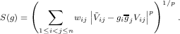 Here Ṽij is the visibility measurement obtained on the i–j baseline (at
a given instant), V ij is the corresponding model visibility, and wij is a
suitably chosen weight. Usually the gk may be assumed not to vary
too rapidly with time, so that one may minimize, instead, the
functional
Here Ṽij is the visibility measurement obtained on the i–j baseline (at
a given instant), V ij is the corresponding model visibility, and wij is a
suitably chosen weight. Usually the gk may be assumed not to vary
too rapidly with time, so that one may minimize, instead, the
functional
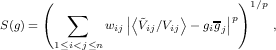 where
where  is the time-average of the ratio of observed visibility
to model visibility, over a time period during which the gk may be
assumed constant.
is the time-average of the ratio of observed visibility
to model visibility, over a time period during which the gk may be
assumed constant.
The AIPS implementation allows the choices p = 1 and p = 2.
Choosing p = 2 yields the least-squares solution for g. When one
chooses p = 1, so that a weighted sum of the moduli of the
residuals is minimized, the computed gain solutions are less
influenced by wild data points, but there is some loss of statistical
efficiency—i.e., the least-squares solutions are superior when the
distribution of measurement errors is well-behaved. (Probably
the choice p ≃ 1.2 would offer a better compromise between
efficiency and robustness). See [F. R. Schwab, Robust solution
for antenna gains, VLA Scientific Memo. No. 136] for further
details.
One may wish to solve only for the antenna/i.f. phases ψk(t) rather
than for the gk if, for example, atmospheric phase corruption is
believed to be the dominant source of systematic error. In this case,
one minimizes
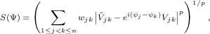 or
the version thereof incorporating time-averages.
or
the version thereof incorporating time-averages.
Cornwell and Wilkinson [A new method for making maps with
unstable radio interferometers, Mon. Not. R. Astr. Soc., 196 (1981)
1067–1086] suggest adding to S terms which arise by assuming
prior distributions for the gk; these “penalty terms” would be
chosen so as to increase in magnitude as the solution parameter
deviates from a prior mean which one might take, say, as the running mean of previous gain solutions. The widths of the prior
distributions could be based on empirical knowledge of the
behavior of the array elements. Such a modification can be useful
when the array is composed of antenna elements of differing
collecting area. This modification is used in order to constrain the
moduli of the computed gains in one version of the AIPS task for
self-calibration which is used primarily for VLBI data reduction
(VSCAL).
Shannon sampling theorem — Suppose the complex-valued
function f of the real variable t to be square-integrable, and
assume that f is band-limited; i.e., that its Fourier transform
 (x) = ∫
-∞∞f(t)e2πixtdt ≡ 0 for |x| > a. Then f is completely
determined by its values at the discrete set of sampling points n∕2a,
n = 0, 1, 2,… , and f can be recovered via the Shannon series (also
called the cardinal series)
(x) = ∫
-∞∞f(t)e2πixtdt ≡ 0 for |x| > a. Then f is completely
determined by its values at the discrete set of sampling points n∕2a,
n = 0, 1, 2,… , and f can be recovered via the Shannon series (also
called the cardinal series)
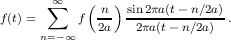 The series converges both uniformly and in the mean-square
sense.
The series converges both uniformly and in the mean-square
sense.
The Shannon series can be derived by expanding  in a Fourier
series, and then applying Fourier inversion—or it can be derived from
the classical Poisson summation formula. It is sometimes referred to as
Whittaker’s cardinal interpolation formula or the Whittaker–Shannon
sampling series, having first been studied in detail by E. T. Whittaker
in 1915 and later introduced into the literature of communications
engineering by Shannon in 1949. By the Paley–Wiener theorem, since f
is band-limited, it can be analytically extended from the real line to the
full complex plane, as an entire function of slow growth. The
Shannon series, which converges for complex as well as real
t, is one means of doing so. Whittaker referred to the series
as “a function of royal blood in the family of entire functions,
whose distinguished properties separate it from its bourgeois
brethren.”
in a Fourier
series, and then applying Fourier inversion—or it can be derived from
the classical Poisson summation formula. It is sometimes referred to as
Whittaker’s cardinal interpolation formula or the Whittaker–Shannon
sampling series, having first been studied in detail by E. T. Whittaker
in 1915 and later introduced into the literature of communications
engineering by Shannon in 1949. By the Paley–Wiener theorem, since f
is band-limited, it can be analytically extended from the real line to the
full complex plane, as an entire function of slow growth. The
Shannon series, which converges for complex as well as real
t, is one means of doing so. Whittaker referred to the series
as “a function of royal blood in the family of entire functions,
whose distinguished properties separate it from its bourgeois
brethren.”
Suppose that f(t) is “small” for |t| > b (no nontrivial signal is both
band-limited and time-limited). Then, assuming that b is integral, the
number of terms in the Shannon series that really matter is 4ab.
This suggests that the space of “essentially band-limited” and
“essentially time-limited” signals has dimension equal to the
time-bandwidth product 4ab. The precise sense in which this is so,
together with a discussion of the prolate spheroidal wave functions (q.v.),
which are relevant to the problem, is described by H. Dym
and H. P. McKean [Fourier Series and Integrals, Academic Press,
New York, 1972] and by David Slepian [Some comments on
Fourier analysis, uncertainty and modeling, SIAM Rev., 25 (1983)
379–393].
The multi-dimensional extension of the sampling theorem to
rectangles implies that if an “unconfused” radio source f(x,y) is
confined to a small region of sky |x| < x0, |y| < y0 (radians),
then it can be reconstructed unambiguously from a discrete set
of visibility samples  (mΔu,nΔv), m,n = 0, 1, 2,…, with
Δu = 1∕2x0 and Δv = 1∕2y0 wavelengths. See cellsize and
Nyquist sampling rate. Other useful extensions of the sampling
theorem—for example, to various multi-dimensional sampling
configurations (e.g., 2–D hexagonal sampling lattices), to the case of
stochastically jittered sampling, to derivative sampling (e.g., in
1–D, f can be recovered from samples of f and its derivatives
through order r taken at intervals (r + 1) n_
2a ), etc.—and sampling
theorems for functions whose transforms of other than Fourier
type are of compact support—are described in survey articles
by A. J. Jerri [The Shannon sampling theorem—its various
extensions and applications: a tutorial review, Proc. IEEE, 65
(1977) 1565–1596] and J. R. Higgins [Five short stories about
the cardinal series, Bull. (New Ser.) Amer. Math. Soc., 12 (1985)
45–89].
(mΔu,nΔv), m,n = 0, 1, 2,…, with
Δu = 1∕2x0 and Δv = 1∕2y0 wavelengths. See cellsize and
Nyquist sampling rate. Other useful extensions of the sampling
theorem—for example, to various multi-dimensional sampling
configurations (e.g., 2–D hexagonal sampling lattices), to the case of
stochastically jittered sampling, to derivative sampling (e.g., in
1–D, f can be recovered from samples of f and its derivatives
through order r taken at intervals (r + 1) n_
2a ), etc.—and sampling
theorems for functions whose transforms of other than Fourier
type are of compact support—are described in survey articles
by A. J. Jerri [The Shannon sampling theorem—its various
extensions and applications: a tutorial review, Proc. IEEE, 65
(1977) 1565–1596] and J. R. Higgins [Five short stories about
the cardinal series, Bull. (New Ser.) Amer. Math. Soc., 12 (1985)
45–89].
Shannon series — See Shannon sampling theorem.
shed — See sub-task.
SIVPSF — See point spread function.
slice — a one-dimensional cut across an image. E.g., the
slice of a two-dimensional image f which passes through
(x0,y0) and has orientation angle ϕ is the sub-image h given by
h(t) = f(x0 + t cos ϕ,y0 + t sin ϕ). In AIPS, a slice may be excised
from an image by issuing the verb command SLICE. Since AIPS deals
only with digitized images, the program must interpolate to obtain
data along the cut, except when the slice is taken along a row or
column of the image.
slice file — in AIPS, an extension file, associated with an image file,
in which a digitized slice (q.v.), or one-dimensional sub-image, of the
primary image is stored. In order to display a slice, one may issue the
verb command SL2PL, which causes AIPS to read the contents of a
slice file and generate a plot file.
snapshot — in earth-rotation aperture synthesis interferometry,
an observation which is of such short duration that Earth’s motion
does not significantly enhance the u-v coverage, or a map derived from
such a brief observation. Compare full-synthesis map.
For a thorough discussion of the use of the VLA in snapshot mode,
see §5 of A. H. Bridle’s Lecture No. 16 in the 1985 Summer School
Proceedings.
software mount — a computer’s reaction to the issuing of a
command to it informing it that the hardware mount of some external
storage module, such as a disk pack or a reel of magnetic tape, has
occurred, and that the computer should open the channel of access to
this module. See hardware mount.
sort order — the ordering of visibility measurements within a u-v
data file. Time-baseline order is convenient for purposes of calibration,
baseline-time order for data display, and so-called x-y order for gridding
and subsequent mapping.
source editor — same as text editor. (Formerly, computers were
used mainly for numerical computations and text editors primarily for
the editing of program source code—hence the name source
editor).
spatial resolution — In digital image analysis, this term refers
rather imprecisely to the minimum size of details which can be
discerned. The spatial resolution is determined by three factors: the
inherent indeterminacy of whatever image reconstruction problem
underlies the method by which the image was produced (and the
properties of the image reconstruction algorithm which produced the
image); the measurement noise; and the pixel size—i.e., the size
of the squares or the rectangles comprising the reconstruction
matrix.
In radio interferometry, the inherent spatial resolution goes
roughly in inverse proportion to the physical size scale D of the array
(measured in wavelengths). For observations at a wavelength λ, the
inherent spatial resolution, with a filled aperture, is essentially λ∕D
radians. However, with a synthesis array with large gaps in
the u-v coverage, the effective resolution is somewhat coarser.
Often, some measure of the spread of the central lobe of the
dirty beam (say, the FWHM) is quoted as the spatial resolution.
However, some reconstruction methods (e.g., the regularization
methods) produce images in which the resolution of bright features
may be much finer than that of dim features. This property of
regularization methods may be viewed as either good or bad: S∕N
dependent spatial resolution complicates the interpretation of an
image, but, on the other hand, one may gain additional contrast
resolution—i.e., low surface-brightness features may become
more readily discernible. An honest statement concerning the
spatial resolution of an image must be based upon empirical
knowledge of the reconstruction method that was used. See
super-resolution.
spawn — See sub-task.
spheroidal function — an eigenfunction ψαn of a finite,
weighted-kernel Fourier transform—more precisely, for given c and
given α > -1, one of the countably many solutions of the integral
equation
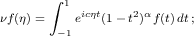 equivalently, a solution of the differential equation
(1 -η2)f′′- 2(α + 1)ηf′ + (b-c2η2)f = 0. The eigenfunction ψα0
of the equation above associated with the largest eigenvalue ν is
termed the 0-order solution. The choice α = 0 of weighting exponent
yields the family
equivalently, a solution of the differential equation
(1 -η2)f′′- 2(α + 1)ηf′ + (b-c2η2)f = 0. The eigenfunction ψα0
of the equation above associated with the largest eigenvalue ν is
termed the 0-order solution. The choice α = 0 of weighting exponent
yields the family 
 of prolate spheroidal wave
functions.
of prolate spheroidal wave
functions.
Weighted 0-order spheroidal functions (1 - η2)αψα0 are optimal
gridding convolution functions in the same sense that the prolate
spheroidal wave functions (q.v.) are optimal, except that now the
weighted concentration ratio
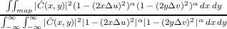 is
maximized (see the paper by F. R. Schwab in the 1983 Sydney
Conference Proceedings). The weighting exponent α is used to trade off
the effectiveness of the aliasing suppression at the edge of the field of
view, against that in the central region of the map. The choice α = 1,
with a support width of six u-v grid cells, yields an effective gridding
convolution function, emphasizing aliasing suppression in the central
region of the map; this function, ψ10, with c = 3π, is the default
function used in the AIPS mapping program. See gridding convolution
function.
is
maximized (see the paper by F. R. Schwab in the 1983 Sydney
Conference Proceedings). The weighting exponent α is used to trade off
the effectiveness of the aliasing suppression at the edge of the field of
view, against that in the central region of the map. The choice α = 1,
with a support width of six u-v grid cells, yields an effective gridding
convolution function, emphasizing aliasing suppression in the central
region of the map; this function, ψ10, with c = 3π, is the default
function used in the AIPS mapping program. See gridding convolution
function.
Stokes’ parameters — the four coordinates relative to a
particular basis for the representation of the polarization state of an
electromagnetic wave propagating through space. Consider a wave
propagating along the z-direction in a right-handed (x,y,z) Cartesian
coordinate system. At a fixed point in space, let the instantaneous
components of the electric field vector, in the x- and y-directions, be
denoted by Ex(t) and Ey(t), respectively; and assume them to be
stationary (in the weak sense, and square-integrable) stochastic
processes. Form the matrix
 Here, the bracketed expressions are expectation values, or correlation
functions, in the lag variable τ, and ^ denotes Fourier transform
with respect to τ. Thus each element of S is a function of frequency ν.
S is Hermitian (conjugate symmetric), owing to the stochasticity
assumptions. The three Pauli spin matrices, together with the 2 × 2
identity matrix, form a basis for the algebra of 2 × 2 Hermitian
matrices; i.e., each such matrix S can be represented in the form
The four (real) coefficients, σ1,…,σ4, of the representation of S in
this basis are called Stokes’ parameters. They commonly are
denoted by I(ν), Q(ν), U(ν), and V (ν), respectively. In other
words,
Here, the bracketed expressions are expectation values, or correlation
functions, in the lag variable τ, and ^ denotes Fourier transform
with respect to τ. Thus each element of S is a function of frequency ν.
S is Hermitian (conjugate symmetric), owing to the stochasticity
assumptions. The three Pauli spin matrices, together with the 2 × 2
identity matrix, form a basis for the algebra of 2 × 2 Hermitian
matrices; i.e., each such matrix S can be represented in the form
The four (real) coefficients, σ1,…,σ4, of the representation of S in
this basis are called Stokes’ parameters. They commonly are
denoted by I(ν), Q(ν), U(ν), and V (ν), respectively. In other
words,
 with I, Q, U, and V real.
Stokes’ parameter I measures the total intensity of the radiation
field, Q and U the linearly polarized intensity, and V the circularly
polarized intensity. I always is non-negative. For a totally unpolarized
wave, Q = U = V = 0; for a partially polarized wave, the ratio
 ∕I measures the total degree of polarization,
 ∕I the degree of linear polarization, and 1
2 arctan U
Q the
orientation angle of the linearly polarized component. Q + iU
is called the complex linear polarization. The IAU and IEEE
orientation/sign conventions have the z-axis directed toward the
observer, the x-axis directed north, and a +i in the argument of the
exponential kernel of the FT. Positive V corresponds to right circular
polarization, and conversely. The polarization response of an
interferometer can be described by forming the so-called cross-spectral
density matrix, which is like the S above but is formed from
measurements of the electric field taken at two points in space.
For further details, including a description of the polarization
response of an interferometer, for various feed configurations,
see Carl Bignell’s Lecture No. 6 in the 1982 Summer Workshop
Proceedings.
∕I the degree of linear polarization, and 1
2 arctan U
Q the
orientation angle of the linearly polarized component. Q + iU
is called the complex linear polarization. The IAU and IEEE
orientation/sign conventions have the z-axis directed toward the
observer, the x-axis directed north, and a +i in the argument of the
exponential kernel of the FT. Positive V corresponds to right circular
polarization, and conversely. The polarization response of an
interferometer can be described by forming the so-called cross-spectral
density matrix, which is like the S above but is formed from
measurements of the electric field taken at two points in space.
For further details, including a description of the polarization
response of an interferometer, for various feed configurations,
see Carl Bignell’s Lecture No. 6 in the 1982 Summer Workshop
Proceedings.
Stokes’ visibility functions — Stokes’ visibility functions, V I,
V Q, V U, and V V , are the Fourier transforms (FT’s) of the radio
brightness (spatial) distributions of Stokes’ parameters, I(x,y), Q(x,y),
U(x,y), and V (x,y). (Here, V I = Î, V Q =  , etc., where ˆ denotes
FT.)
, etc., where ˆ denotes
FT.)
For a radio interferometer with ideal circularly polarized feeds, the
relations between Stokes’ visibility functions and the visibilities, V RR,
V LL, V RL, and V LR, obtained by correlating right circular
response with right, left with left, etc., are V I = 1
2(V RR + V LL),
V Q = 1
2(V LR + V RL), V U = i
2(V LR-V RL), V V = 1
2(V RR-V LL).
Note that each of Stokes’ visibility functions is Hermitian. On the
assumption that circular polarization is absent (i.e., that V (x,y) ≡ 0),
V RR is equal to V LL, and both are Hermitian.
Components of the systematic errors affecting visibility
measurements are i.f.-dependent; hence VLA u-v data files usually do
not contain Stokes’ visibilities, but rather V RR, V LL, V RL, and
V LR—as these are what is required for calibration purposes. Stokes’
visibility functions generally are constructed only within the mapping
programs. (But the AIPS visibility data format is designed to
accommodate either type of visibility function, and the map making
tasks are able to recognize the form of their input data and deal with
them appropriately.)
sub-image — in AIPS parlance, any linear, rectangular, or
hyper-rectangular section of an image.
sub-task — a task, or computer program, whose execution is
initiated by the action of another program. The act of initiating the
execution of the sub-task is called task shedding or task spawning. See
task.
super-resolution — The problem of image reconstruction in
radio interferometry is one of finding an approximation to an
unknown function f (generally assumed to be of compact support) from
partial knowledge of its Fourier transform  — i.e., from a finite
number of measurements of the visibility. Any of the techniques which
are applied to the problem—the Högbom Clean algorithm, the
regularization method, etc.—may be thought of as methods of
smoothing, interpolating, and extrapolating the noisy measurements.
Super-resolution is a term which refers to the extrapolation aspect:
Cautious extrapolation yields an image whose spatial resolution is
≈ λ∕D, where D is the diameter of the largest centered region in the
u-v plane which has been reasonably well sampled. Less cautious
extrapolation yields super-resolution; spurious detail appears as
caution is abandoned.
— i.e., from a finite
number of measurements of the visibility. Any of the techniques which
are applied to the problem—the Högbom Clean algorithm, the
regularization method, etc.—may be thought of as methods of
smoothing, interpolating, and extrapolating the noisy measurements.
Super-resolution is a term which refers to the extrapolation aspect:
Cautious extrapolation yields an image whose spatial resolution is
≈ λ∕D, where D is the diameter of the largest centered region in the
u-v plane which has been reasonably well sampled. Less cautious
extrapolation yields super-resolution; spurious detail appears as
caution is abandoned.
Super-resolution in a Clean map is effected by choosing an
artificially narrow Clean beam. With regularization methods (in image
reconstruction, and more generally), super-resolution comes about by
choosing a small value of the regularization parameter. The spatial
resolution achieved by a regularization method may be signal-to-noise
dependent—bright features may be super-resolved, and dim ones
not.
support — The closure of that subset of the domain of definition
of a function f (or of a generalized function, or distribution) on which
the function assumes a nonzero value is called the support of the
function, and is denoted by supp(f). I.e., supp(f) = 
 .
.
For example, the support of the function f(x) = x is the whole real
line, even though f(0) = 0. And the support of
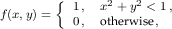 is
the closed unit disk,
is
the closed unit disk, 
 .
.
In Euclidean space, a function f whose support is bounded—i.e.,
such that f ≡ 0 “far-out”—is said to be of compact support. The Fourier
transform of a nontrivial function of compact support (such as a u-v
measurement distribution or a gridding convolution function) cannot
itself be of compact support; i.e., it has “sidelobes” extending to
infinity.
support width — of a function whose support is a rectangle or a
hyper-rectangle (e.g., the Fourier transform of a band-limited
function), the linear measure of one of the edges of its support.
SVPSF — See point spread function.
Synthesis Imaging in Radio Astronomy — A collection of
lectures from the 1988 (Third) NRAO Synthesis Imaging Summer
School edited by R. A. Perley, F. R. Schwab and A. H. Bridle.
(Astronomical Society of the Pacific Conference Series, Volume 6
(1989)). A very useful reference book for the reduction of radio
interferometric data. This volume supersedes the proceedings from
the earlier workshops.
synthesized beam — in radio interferometry, the beam—but
always ignoring instrumental effects. Hence, the synthesized beam is
fully determined by the u-v sampling distribution, the u-v weight
function, the u-v taper function, and the gridding convolution function. See
beam.
tape blocking efficiency — Data are stored on magnetic
tape in units of blocks. An inter-record gap—essentially wasted
space—separates one block from the next. The tape blocking efficiency,
or the fraction of unwasted space, is the ratio
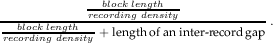 The length of an inter-record gap is about 3
4 , 3
5 , and 3 _
10 inch at
recording densities of 800, 1600, and 6250 bpi, respectively.
The length of an inter-record gap is about 3
4 , 3
5 , and 3 _
10 inch at
recording densities of 800, 1600, and 6250 bpi, respectively.
taper — See u-v taper function.
task — used in two senses: 1) the execution of a computer
program and 2) the program itself. Thus, if two computer users are
(independently) running the same program at the same time, it may
be said either that two tasks are running, or that two incarnations of
the same task are in existence. A sub-task (q.v.) is a task whose
execution is initiated by the action of another program. Many of the
more complicated and the more specialized functions of AIPS are
accomplished by the action of sub-tasks shed by the AIPS program.
(Simpler functions are invoked by the issuance of verb commands—see
POPS symbols.)
t-b order — See time-baseline order.
TEK screen — a cathode ray tube (CRT) terminal and display
device appropriate for pictorial display of data, in the form of contour
plots, graphs, etc., as well as for display of textual data. The Tektronix
company’s Model 4012 terminal (with a green P4 phosphor, hence the
synonymous term green screen) is the canonical device of this type. The
“make copy” button on this device can be used to produce a copy,
on paper, of the image shown on the CRT screen. Each of the
NRAO’s AIPS data reduction computers is outfitted with a TEK
screen.
TEK4012 — same as TEK screen.
Telex 6250 tape drive — a model of tape drive used on the VLA
Vaxes, capable of operation at 1600 and 6250 bpi.
terminal page — Many modern computer terminals contain a
semiconductor memory with a capacity of several CRT screen loads
(≈ 24 lines) of character data. A terminal page is a unit of one screen
load of such data. Certain terminal keys allow one to cause data which
previously appeared on the CRT screen to reappear—this feature is
called terminal scroll (q.v.). A typical terminal at the NRAO has three
terminal pages of memory.
terminal scroll — that feature present on certain models of
computer terminals which allows data which previously appeared on
the CRT screen to be made to reappear. Often, depressing one key on
the terminal will cause earlier information to reappear line-by-line
(this is termed line scroll), while the action of another key will
cause a whole earlier screen load to reappear (this is termed page
scroll).
text editor — a computer program designed for the creation,
manipulation, and modification of computer files containing textual
data such as reports, documentation, alphanumeric command lines,
and program source code. Generally, one or more text editors are
supplied by the computer manufacturer. Three text editors are in
widespread use on the Vax—SOS, EMACS and EDT. vi, edt and emacs
are used on NRAO’s Convex computers. See line editor and screen
editor.
text file — a computer data file containing only textual data, as
might be written by a text editor (q.v.). Programs such as the AIPS tasks
sometimes write messages, especially progress report messages, into a
text file—see message file.
Third NRAO Synthesis Imaging Summer School — The
1988 Summer School on Synthesis Imaging which was held in Socorro,
New Mexico in June 1988. The lectures were formally published in
Synthesis Imaging in Radio Astronomy.
thrashing — See memory thrashing.
time-baseline order — An ordered set of visibility measurements

 recorded with an n
element interferometer at times t1 < t2 < … < tl is said to be in
time-baseline order if the ordering is such that all of the data obtained at
time t1, sorted into the canonical ordering by baseline, occur
first, followed by the data obtained at time t2, again ordered
canonically, etc., etc. (The canonical ordering by baseline is the order
V 12,V 13,…,V 1n,V 23,…,…,V n-1,n .) Compare baseline-time
order.
recorded with an n
element interferometer at times t1 < t2 < … < tl is said to be in
time-baseline order if the ordering is such that all of the data obtained at
time t1, sorted into the canonical ordering by baseline, occur
first, followed by the data obtained at time t2, again ordered
canonically, etc., etc. (The canonical ordering by baseline is the order
V 12,V 13,…,V 1n,V 23,…,…,V n-1,n .) Compare baseline-time
order.
Time-baseline ordering of a u-v data file is convenient for
calibration purposes. The AIPS task for self-calibration requires that its
input u-v data file be time-baseline ordered.
time smearing — in a radio interferometer map, the space-variant
broadening of the point spread function (or beam) which is due to time
averaging of the data. When, for example, the visibility data along a
u-v track are averaged, with equal weight, over time intervals of width
Δt sec., the visibility amplitude of a point source is reduced by a factor
≈ sin γ
γ —where γ ≡ π(u′x + v′y + w′z)Δt, where the primes denote
the time rate of change of the spatial frequency coordinates (u,v,w)
along the track (wavelengths/sec.), and where (x,y,z) denotes the
direction cosines of the location of the point source with respect to the
phase tracking center. For further details, see A. R. Thompson’s Lecture
No. 2 and Alan Bridle and Fred Schwab’s Lecture No. 13 in the Third
NRAO Synthesis Imaging Summer School. Compare bandwidth
smearing.
trackball — a spherical ball mechanism, about the size (10 cm., or
so, in diameter) of a tennis ball, which may be oriented manually by
the interactive user of a television display device such as the I2S. The
ball can be rotated about any axis, and its orientation, which is sensed
by the computer, typically is used to control the enhancement or the
coloration of the displayed data (i.e., to control the TV transfer
function(s)), or to position the TV cursor, in order to point out to a
program features in the displayed image which are of particular
interest.
trackball button — On the unit which houses the trackball
for the I2S Model 70 TV display device are the four trackball
buttons, labeled A, B, C, and D. These are switches that are used,
in conjunction with the display routines, to exert additional
control over the TV display. Occasionally these buttons are put to
other use in AIPS, such as stopping the Clean deconvolution
program.
transfer function — a transform which can be used to describethe output of a device (say, an electrical transducer) as a function of
the input to the device. See TV look-up table.
TRC — top right corner, the corner of an image diagonally
opposite the BLC. See m × n map.
true color display — a type of false color display, (q.v.).
TU77 tape drive — a model of tape drive used on the NRAO’s
Vaxes, capable of operation at 800 and 1600 bpi.
TU78 tape drive — a model of tape drive used on the VLA
Vaxes, capable of operation at 1600 and 6250 bpi.
TV blink — a feature of a computer-controlled TV display
device, such as the I2S, intended to facilitate the comparison of a pair
of images stored on two different image planes. The TV display is made
to alternate between the two images. The AIPS implementation of
blinking allows the user, by manipulating the trackball, to control the
rate of alternation and the fraction of time that each image is
displayed.
TV cursor — See crosshair.
TV image catalog — See image catalog.
TV look-up table — a memory within the control unit of
a TV display device which is used for storage of the transfer
functions controlling the intensity of the display, as a function of
pixel value. Within AIPS, the transfer functions may be altered
through the use of interactive verbs and manipulation of the
trackball.
TV roam — a feature of a computer-controlled TV display device
such as the I2S which allows contiguous parts of a single large
image, stored on more than one image plane, to be displayed as if
the image were stored on a single, larger image plane. On the
I2S unit, the portion of the image to be displayed on the TV
screen is selected by manipulation of the trackball. See image
plane.
TV scroll — a feature of a computer-controlled TV display
device such as the I2S which allows the display of an image stored
on a single image plane to be moved about the display screen.
This feature, which also is called panning, commonly is used in
combination with the TV zoom capability. On the I2S unit, the scroll
ordinarily is controlled by manipulation of the trackball. Compare TV
roam.
TV zoom — a magnification feature of a computer-controlled TV
display device such as the I2S. On the I2S, the three available
magnification factors (which multiply the linear dimensions of the
original display of the image by a factor of 2, 4, or 8) generally are
selected by depressing one of the trackball buttons. Since the
magnification is achieved by pixel replication (i.e., by piece-wise linear
interpolation)—rather than by a smooth interpolation—the visual
impression may be somewhat displeasing. The entire magnified image
may not fit on the TV screen, so zoom usually is used in combination
with the TV scroll feature.
uniform weighting — A dirty map obtained by computing the
inverse Fourier transform (FT) of a weighted u-v measurement
distribution in which each visibility sample has been weighted in
inverse proportion to the local density of the u-v coverage is said to
have been computed using uniform weighting. When a radio map is
computed via the fast Fourier transform algorithm, uniform weighting
may be achieved by computing normalized discrete convolution
summations ∑
i=1NC(u-ui,v -vi)Ṽi∕N, where (u,v) denotes the
spatial frequency coordinates of a given u-v grid cell, where C is an
appropriately chosen gridding convolution function, and where the Ṽi
are the N visibility measurements obtained at positions (ui,vi) in
some neighborhood of (u,v), the size of which is determined by the
support of C. The uniform weighted map is given by the inverse
discrete FT of data interpolated and smoothed in this manner, onto the
lattice points of a rectangular grid. So-called natural weighting is
achieved by using unnormalized convolution sums, rather than by
dividing by N. The AIPS map making tasks use a weighting
scheme which is slightly more complicated than that described
here.
Since the density of u-v coverage typically is greater in the
inner regions of the u-v plane, a map computed using uniform
weighting has finer spatial resolution than one computed with
natural weighting. With natural weighting, low surface-brightness
extended features may be more easily discernible than with uniform
weighting. Essentially the same effect can be achieved with
uniform weighting, when accompanied by use of a u-v taper
function.
UNIX — a “universal” computer operating system developed at
the Bell Telephone Laboratories. Its virtue is that program packages
such as AIPS—once having been made to run under one UNIX-based
operating system—ought to run on any other such system, even on a
computer of different manufacture, with no alterations. Many Vaxes
operate under UNIX, though not the NRAO’s. The Convexes C-1 in
Charlottesville and at the AOC operates under UNIX. See operating
system.
user-coded task — an AIPS task written by a user, rather than by
a professional programmer or a member of the AIPS programming
group. One of the design goals for AIPS, not yet fully realized, is that it
should be relatively easy for a user who is not an experienced
programmer to write an AIPS task suited to his own needs—i.e., that
it should be fairly simple for him to make some sense of the
AIPS database, and to get at his data and manipulate it as he
sees fit. The AIPS task named FUDGE is intended to serve as a
paradigm for user-coded tasks for manipulation of u-v data files; two
other tasks, TAFFY and CANDY, are paradigms for image file
manipulation. A useful reference is the manual by W. D. Cotton and a
‘cast of AIPS’ [Going AIPS! A Programmers Guide to the NRAO
Astronomical Image Processing System, NRAO, Charlottesville, VA,
1990].
The addition to AIPS of new verbs, and modification of the
functioning of existing verbs, requires modifying the AIPS program
itself; this is best left to the AIPS programming group.
u-v coverage — the support of the u-v sampling distribution (q.v.).
Also see conjugate symmetry.
u-v data file — in AIPS, a primary data file designed to
accommodate the measurements of the visibility function of a radio
source.
u-v data flag — In an AIPS u-v data file, each visibility
measurement is accompanied by a real-valued weight, which
ordinarily is (positive and) proportional to the length of the
integration period over which the measurement was obtained. A
non-positive weight represents a u-v data flag, which signifies that the
visibility measurement ought to be ignored. See flagging and
clipping.
u-v FITS format — an extension of the FITS format
(originally designed for the interchange of image data) to
accommodate radio interferometer visibility data [E. W. Greisen and
R. H. Harten, An extension of FITS for groups of small arrays of
data, Astron. Astrophys. Suppl. Ser., 44 (1981) 371–374]. See FITS
format.
u-v measurement distribution — in radio interferometry, a
linear combination of shifted Dirac δ-functions, one located at
the position in the u-v plane of each visibility measurement,
and each weighted by the visibility measurement obtained at
that location. Denoting the u-v coverage by {(ui,vi)}i=1n, the
visibility function by V , and the measured visibility by Ṽ, the
(two-dimensional) u-v measurement distribution S is given by
S(u,v) = ∑
i=1nṼ(ui,vi)δ(u - ui,v - vi). Compare u-v sampling
distribution.
This definition may be modified to incorporate two types of
weight function, yielding a weighted and/or tapered measurement
distribution—see u-v taper function and u-v weight function.
The visibility measurements {Ṽ(ui,vi) } are not actual samples of
V , but rather are error-corrupted samples of a function which
represents some sort of local average of the visibility—this is a
distinction which it is worthwhile to note, and then to ignore. Various
systematic errors affecting the measurements may be corrected
by proper calibration—see antenna/i.f. gain and instrumental
polarization.
u-v sampling distribution — in radio interferometry, a linear
combination of shifted Dirac δ-functions, one located at the position in
the u-v plane of each visibility measurement. Sometimes termed u-v
transfer function. See beam.
If {(ui,vi)}i=1n (the u-v coverage) is the set of spatial frequency
coordinates at which the source visibility has been sampled, then
the (two-dimensional) u-v sampling distribution S is given by
S(u,v) = ∑
i=1nδ(u - ui,v - vi).
Occasionally the term u-v sampling distribution is used in the same
sense as the term u-v measurement distribution (q.v.).
u-v taper function — an even, real-valued weight function
(typically, an elliptical Gaussian), smooth and peaked at the
origin, which may be incorporated into the definition of u-v
measurement distribution or u-v sampling distribution, above, serving to
control the spatial resolution of the radio map or the beam; i.e., to
enhance the response to extended features in the radio source
brightness distribution by giving relatively higher weight to
the measurements at short u-v spacings. Compare u-v weight
function.
u-v transfer function — same as u-v sampling distribution, but
always explicitly incorporating any u-v weight function or u-v taper
function.
u-v weight function — a real-valued function which may be
incorporated in the definition, above, of u-v measurement distribution or
u-v sampling distribution, serving to weight each measurement either
according to an estimate of the statistical measurement error, or
according to the local density of sampling, or both. Compare u-v taper
function and see uniform weighting.
Varian printer — an electrostatic printer/plotter manufactured
by the Varian Corp.
Variational Method — the name which applies to Tim
Cornwell’s AIPS implementation (in the program VM) of the maximum
entropy method, to solve the image deconvolution problem g = b * f,
where g and b are given, and f is unknown. The regularizing
term S( ) (see regularization method), a function of the computed
approximate solution
) (see regularization method), a function of the computed
approximate solution  , is given by the negative of an entropy
expression, of the form
, is given by the negative of an entropy
expression, of the form
 Here A denotes the (assumed known) support of f, and h is a prior
estimate of f; when h ≡ constant, this agrees with the standard
formulation of the maximum entropy method. A weighted sum
χ2(
Here A denotes the (assumed known) support of f, and h is a prior
estimate of f; when h ≡ constant, this agrees with the standard
formulation of the maximum entropy method. A weighted sum
χ2( ) + λS(
 ) of a χ2 error term and S is minimized, and the
regularization parameter λ is chosen so that the r.m.s. residual
corresponding to the final iterate is approximately equal to an input
value. For optical data the χ2 term is taken as ∥g - b *
) of a χ2 error term and S is minimized, and the
regularization parameter λ is chosen so that the r.m.s. residual
corresponding to the final iterate is approximately equal to an input
value. For optical data the χ2 term is taken as ∥g - b * ∥2, whereas
for radio data the χ2 term is evaluated in the visibility domain, where
the measurement errors may more properly be assumed to be
statistically independent. Also, ∫
A
∥2, whereas
for radio data the χ2 term is evaluated in the visibility domain, where
the measurement errors may more properly be assumed to be
statistically independent. Also, ∫
A is constrained to be near an
estimate of the zero-spacing flux which is supplied by the user. The
minimization is done using a Newton-type method, with a diagonal
approximation to the Hessian of the objective function and intricate
control of the step length. In terms of execution speed, this method is
competitive with the Clark Clean algorithm—at least in the case of
large objects of complex structure observed with the VLA—and
superior results usually are obtained for this class of objects. See
[T. J. Cornwell, Deconvolution with a maximum entropy type
algorithm, VLA Scientific Memo. No. 149].
is constrained to be near an
estimate of the zero-spacing flux which is supplied by the user. The
minimization is done using a Newton-type method, with a diagonal
approximation to the Hessian of the objective function and intricate
control of the step length. In terms of execution speed, this method is
competitive with the Clark Clean algorithm—at least in the case of
large objects of complex structure observed with the VLA—and
superior results usually are obtained for this class of objects. See
[T. J. Cornwell, Deconvolution with a maximum entropy type
algorithm, VLA Scientific Memo. No. 149].
verb — See POPS symbols.
Versatec printer — an electrostatic printer/plotter manufactured
by the Versatec Corp., and used on the NRAO’s AIPS computer
systems.
Very Long Baseline Interferometry — Techniques and
Applications — Proceedings of the NATO Advanced Study Institute
held at Castel S. Pietro Terme, Bologna, Italy in 1988. Edited by
M. Felli and R. E. Spencer. Kluwer Academic Publishers, Dordrecht
(1989). This volume contains much useful information on the planning
and execution of VLBI observations as well as on the reduction of
VLBI data.
vi — a moderately sophisticated text editor (a screen editor) used
on computers which run the UNIX operating system. See text
editor.
virtual memory page — on a computer running under a virtual
memory operating system, one unit of virtual memory storage. At a
typical Vax installation, the size of a virtual memory page is 512
bytes.
virtual memory page swapping — on a computer running
under a virtual memory operating system, the action (initiated
automatically by the operating system) of reading new virtual
memory pages into the physical memory, and storing on disk (i.e., in
the virtual memory) the data which thus have been displaced. Each
occurrence of the displacement of a memory page is referred to as a
page fault. See memory thrashing.
virtual memory storage — computer storage—typically
disk storage—in an area apart from the physical memory of a
computer. Access to virtual memory storage is controlled by the
operating system, in a way intended to give the programmer
the illusion that a large amount of physical memory is present.
Access to virtual memory may be much slower than access to
physical memory, and the operating system may incur a significant
amount of overhead in managing the virtual memory. See memory
thrashing.
visibility phase tracking center — In a correlating-type radiointerferometer usually the fringe stopping center and the delay tracking
center coincide. When this is the case, both are referred to as the
visibility phase tracking center.
VM — See Variational Method.
VMS — (Virtual Memory System) the operating system used on
the NRAO’s Vax computers. See virtual memory storage and operating
system.
wedge — a legend, or scale—generally in the form of a bar graph
with gradations in intensity and chromaticity—which may be displayed
adjacent to a photographic or video display of a digitized image. The
wedge is a visual representation of the transfer function that was used
in generating the display. The wedge is either colored or gray,
depending on whether the display is a pseudo-color display or a
gray-scale display.
Note that a false color display would require more than one wedge
(or a multi-tiered wedge) to display the several transfer functions,
as well as an additional wedge to display the possible color
mixtures.
window Clean — an application of the Högbom Clean algorithm,
with an explicit specification, by the user, of the Clean window.
Generally the user should specify a Clean window whenever it is
possible to make a reasonably valid and restrictive estimate of the
support of the true radio source brightness distribution. At the
termination of the algorithm, it is prudent to examine a display of the
residual map for the presence of large residuals outside of the Clean
window; their presence could suggest that an inappropriate window
was selected. See Clean window.
working set size — on a computer running under a virtual
memory operating system, the amount of physical memory allocated to
a task. Any program memory requirement in excess of the working set
size is relegated to virtual memory storage. At a typical Vax installation,
the working set size is set at 1
4 or 1
2 megabyte.
x-y order — An ordered set of visibility samples {V (ui,vi,wi)}i=1n
arranged according to descending absolute value of the spatial
frequency coordinate u — i.e., with |u1|≥|u2|≥… ≥|un| — is said
to be in x-y order.
x-y order is a convenient ordering for the operation of gridding
convolution; hence the AIPS mapping tasks require that their input
u-v data files be sorted accordingly. See sort order.
Y-routine — in AIPS, a subroutine designed to aid in the
use of a specific model of TV display device, such as the I2S
Model 70. AIPS requires a relatively small core of Y-routines
implementing basic TV display functions; complicated display
functions then are accomplished by combining these basic functions
that are supposed to be common to many models of TV display
device. At present there are approximately 25 Y-routines for
use at those AIPS installations equipped with an I2S. Compare
Z-routine.
zero-spacing flux — The visibility V (u,v) ≡ (u,v) (
  denotes Fourier transform) of a source brightness distribution f in a
neighborhood of u = v = 0 is inaccessible to an interferometer
composed of elements of finite collecting area. The zero-spacing flux is
equal to the total, or integrated flux density of the source—i.e., it is
given by V (0, 0) = ∫
-∞∞∫
-∞∞f(x,y) dxdy . Because the hole
in the u-v coverage in the neighborhood of the origin may be
fairly large, image reconstruction methods, such as the Högbom
Clean algorithm, may do a poor job, within this central region, of
interpolating the measured data. This frequently is manifested by the
appearance of a negative bowl artifact—a negative ‘baseline’ beneath
the reconstruction of f —owing to the reconstruction method
having underestimated the zero-spacing flux. The Variational
Method for maximum entropy reconstruction requires that the user
supply an estimate of V (0, 0). The Clean algorithm, too, may
benefit if a datum at u = v = 0 is included when the dirty map is
constructed.
denotes Fourier transform) of a source brightness distribution f in a
neighborhood of u = v = 0 is inaccessible to an interferometer
composed of elements of finite collecting area. The zero-spacing flux is
equal to the total, or integrated flux density of the source—i.e., it is
given by V (0, 0) = ∫
-∞∞∫
-∞∞f(x,y) dxdy . Because the hole
in the u-v coverage in the neighborhood of the origin may be
fairly large, image reconstruction methods, such as the Högbom
Clean algorithm, may do a poor job, within this central region, of
interpolating the measured data. This frequently is manifested by the
appearance of a negative bowl artifact—a negative ‘baseline’ beneath
the reconstruction of f —owing to the reconstruction method
having underestimated the zero-spacing flux. The Variational
Method for maximum entropy reconstruction requires that the user
supply an estimate of V (0, 0). The Clean algorithm, too, may
benefit if a datum at u = v = 0 is included when the dirty map is
constructed.
A zero-spacing estimate can be derived from single-dish
measurements. Providing a proper estimate is difficult, because of
contamination of single-dish measurements by ‘confusing sources.’
The estimate ought to correspond to a telescope with the same
primary beam response as the array elements; and it is not just a single
datum V (0, 0) which is missing, but rather a region—so proper
weighting of the zero-spacing information is tricky. See Tim Cornwell
and Robert Braun’s Lecture No. 8 in the Third NRAO Synthesis Imaging
Summer School.
zoom — See TV zoom.
Z-routine — in AIPS, a subroutine—generally designed to
perform some routine, often needed function—written for a
specific model of host computer or for a specific host computer
operating system. The implementation of certain basic functions,
especially those for file access and file management, generally
is machine dependent and operating system dependent. The
typical AIPS installation requires 50–100 Z-routines. Compare
Y-routine.
1978 Groningen Conference Proceedings — Image Formation
from Coherence Functions in Astronomy. Proceedings of IAU Colloquium
No. 49 held at Groningen, the Netherlands, August 10–12, 1978, edited by
C. van Schooneveld, D. Reidel, Dordrecht, Holland, 1979—contains
many papers on aperture synthesis techniques, including some of the
early papers on hybrid mapping.
1982 Summer Workshop Proceedings — Synthesis
Mapping. Proceedings of the NRAO–VLA Workshop held at Socorro,
New Mexico, June 21–25, 1982, edited by A. R. Thompson and
L. R. D’Addario, NRAO, Green Bank, WV, 1982—a collection of the
fifteen lectures which comprised this short course on aperture
synthesis techniques—a useful introduction to VLA data reduction
methods.
1983 Sydney Conference Proceedings — Indirect Imaging:
Measurement and Processing for Indirect Imaging. Proceedings of an
International Symposium held in Sydney, Australia, August 30–September
2, 1983, edited by J. A. Roberts, Cambridge Univ. Press, Cambridge,
1984—contains a number of interesting papers on aperture synthesis
techniques.
1985 Summer School Proceedings — lecture notes from the
second NRAO summer short course on radio-interferometric imaging
(in preparation). This volume supersedes the 1982 Summer Workshop
Proceedings.
1988 Summer School Proceedings — lecture notes from the
third NRAO Summer School on radio interferometric imaging. The
lectures have been published as Synthesis Imaging in Radio Astronomy
(q.v.).
4012 — See TEK screen.