9.7 Self-calibration, imaging, and model-fitting
We are now in a position to make images. As with VLA data, we do this by iteratively self-calibrating the data and
deconvolving using Clean, MEM et al. We describe below a typical self-calibration and imaging sequence for VLBI
data. The tasks used are described in more detail in Chapter 5.
- CALIB self-calibrates the uv data.
- IMAGR images and Cleans. IMAGR is now the preferred task for imaging VLBI data in


 .
.
- SCMAP images, Cleans, and self-calibrates. SCMAP is meant to provide the functionality of the popular
VLBI data analysis package difmap. SCIMG is a multi-field version of SCMAP.
The main difference between the processing of VLBI and VLA data is that, unless phase-referencing is used,
absolute phases of VLBI data are un-calibrated. Therefore, many more iterations around the imaging loop are
required for the VLBI case; dozens of self-calibration iterations are not uncommon. Given this, it may be convenient
to use tasks SCMAP or SCIMG which cycle between imaging and self-calibration with an option to edit the UV data. If
you wish to edit the Clean components or make plots, you will need to do the manual Clean/self-cal process with
IMAGR and CALIB.
Note that VLBI imaging is not an exact science and there are a number of different views on the “correct” imaging
method and the “correct” software to accomplish this method. Some users take their data into a package
written at CalTech to use the difmap program (see ftp://phobos.caltech.edu/pub/difmap/). Others use the
tasks SCMAP and SCIMG (see §5.4). It is beyond the scope of this document to explain in detail all aspects of
VLBI imaging. For more details, see Craig Walker’s chapter on “Practical VLBI Imaging” in the publication VLBI
and the VLBA, 1995, edited by A. Zensus, P.J. Diamond, and P.J. Napier which is available on the World-Wide Web
(www.cv.nrao.edu/vlbabook). Here we make a few suggestions on how to control CALIB and IMAGR.
Again, please note that the latter is preferable to all previous imaging tasks; SCIMG and to a lesser extent
SCMAP offer the same improved imaging techniques. They do not offer several experimental algorithms
found in IMAGR including Clean component filtering, the SDI Clean algorithm, and multi-resolution
Cleaning.
9.7.1 CALIB
- Start by correcting antenna phases only, i.e., use SOLMODE = ’P’ C R. Switch on the amplitude
correction only after you have converged to a fairly good image. On the first iteration, you will
need to invent an input model. For most extragalactic continuum sources, a point-source model is a
good choice. Set SMODEL(1) to the zero-spacing flux density as extrapolated by eye using UVPLT and
consider using a circular Gaussian model at the origin to reduce the impact of the longest spacings.
Start with the so-called SNR parameter APARM(7) small (≤ 1) and gradually increase it as the image
improves. If this parameter is large during early iterations, when the model used is far from correct,
then large portions of your data in the output file may be flagged. This is not too important if you use
the original input uv file as the input to CALIB in all iterations. You can also set APARM(9) = 1 to leave
data affected by failed solutions uncalibrated.
- On subsequent iterations, use the Clean image as produced by IMAGR as your input model. VLBI
applications usually require Clean components well beyond the first negative component to be used
in calculating the source model. One possibility is to use PRTCC to find the point where a significant
fraction (e.g., one third) of all new Clean components are negative. An alternative is to use all of the
Clean components, but to use tight windowing in IMAGR — which can now be done interactively on
the TV as IMAGR progresses. Alternatively, use tight windowing and clipping of the Clean components
in IMAGR (IMAGRPRM(8) and IMAGRPRM(9)) or afterward with CCEDT or CCSEL before running CALIB.
Tight windowing is especially important when uv coverage is poor. Editing Clean components after
IMAGR, but before CALIB, can be effective in removing possibly spurious features; if they are real
they will usually reappear in later iterations. IMAGR offers a filtering option to remove weak, isolated
components when requested from the TV and at the end before the components are restored to the
image. This removes much of the need for CCSEL.
- When carrying out the next CALIB iteration with the new Clean model, you can either self-calibrate
the original data set or, alternatively, self-calibrate the data set (output by CALIB) which was used to
produce that Clean model. It is advantageous to use the original data set at least until you turn on
amplitude calibration. At that point, you should stick with the file produced from the original data
with the best phase-only solution. Amongst other things, this can prevent the telescope amplitudes
from “wandering” (see below).
- When the model contains extended structure, there may be problems with convergence when
weighting the data “correctly” (i.e., by 1∕σ2.) The WEIGHTIT adverb allows you to use less extreme
weights, such as 1∕σ or 1∕
 . If your array contains antennas that have a wide range of sensitivities,
e.g., the VLBA plus the phased-VLA and/or the Effelsberg 100-m, it is helpful to alter the weights of
the antennas in your CALIB solutions. If this is not done, then your solution will be dominated by only
a few baselines and the uniqueness of the solution is not guaranteed. Use PRTUV to inspect the weights
of your data. Then set the CALIB input array ANTWT, which provides multiplicative factors adjusting
the weights for each antenna prior to the CALIB solution. Set these parameters so that the effective
range of baseline weights is only 10 to 100. Alternatively, use WTMOD to raise the original weights to a
power between 0.25 and 0.5.
. If your array contains antennas that have a wide range of sensitivities,
e.g., the VLBA plus the phased-VLA and/or the Effelsberg 100-m, it is helpful to alter the weights of
the antennas in your CALIB solutions. If this is not done, then your solution will be dominated by only
a few baselines and the uniqueness of the solution is not guaranteed. Use PRTUV to inspect the weights
of your data. Then set the CALIB input array ANTWT, which provides multiplicative factors adjusting
the weights for each antenna prior to the CALIB solution. Set these parameters so that the effective
range of baseline weights is only 10 to 100. Alternatively, use WTMOD to raise the original weights to a
power between 0.25 and 0.5.
- As you iterate, keep an eye on how the model image is converging to fit the data. Use VPLOT, CLPLT,
CAPLT, and UVPLT.
- When your source has a lot of extended structure and/or your VLBI array has relatively few short
spacings, you should consider setting UVRANGE to only include the range of spacings in which the
model provides a good fit to the data. However, given the relatively small number of antennas in most
VLBI observations, you may need to compromise to allow in enough baselines to get good self-cal
solutions. Set WTUV > 0.
- When you are finally ready to solve for amplitude corrections, you should first apply all previous
phase calibration including the final phase-only self-calibration solution. Then run CALIB setting
SOLMOD ’A+P’, initially setting the solution interval (SOLINT) to a longer time than used for phase-only
solutions (e.g., 3 times). Try to prevent the antenna amplitudes from “wandering,” which can
sometimes happen if there is still a significant amount of short spacing flux density missing from the
source model. Setting UVRANGE is useful, as is setting CPARM(2) = 1 to constrain the mean amplitude
solutions over all antennas to be one. You can also set SOLMODE=’GCON’ and the array GAINERR to the
expected standard deviation of the gains for each antenna. This constrains amplitude solutions to
conform to the expected statistics. Setting the gain constraint factor SOLCON to values larger than 1 will
increase the importance of these gain error constraints. Finally, going back and self-calibrating starting
with the original data set and the best available Clean model is useful way to prevent amplitude
wander.
CALIB has been enhanced to improve its usefulness for SVLBI data sets. This has involved the implementation of
improved antenna selection and partial array calibration, through the new adverb DOFIT. The possibility of solving
only for a subset of selected antennas has been implemented in this manner and may prove useful for SVLBI
data. The implementation of adverb DOFIT in CALIB is analogous to its implementation in FRING (see
§9.5.7.7).
9.7.2 IMAGR, SCIMAG, and SCMAP
- Before using IMAGR or SCMAP or SCIMG, print out and read the EXPLAIN file. They are powerful and
complicated tasks with many adverbs — some of which are new — and shouldn’t be used blindly.
- The quality of images produced may depend on the type of weighting used. With VLBA-only
experiments, the best quality images are often produced using natural (UVWTFN ’NA’ C R) weighting
in IMAGR. These images will represent the extended structure of the source better. If the
highest resolution is required, try uniform (UVWTFN ’UN’ C R) weighting. The ROBUST parameter
allows weightings intermediate between these two extremes often with both good signal-to-noise
characteristics and a narrow synthesized beam. It may also be worth experimenting with the UVBOX
parameter to allow smoothing of weights over larger areas of the uv plane (i.e., to use “super-uniform
weighting”). If the array contains antennas with very different sensitivities, (for instance, if it includes
Effelsberg, the phased-VLA, and/or HALCA), then it may be advantageous to alter the weights of
baselines to these antennas. Although this increases the thermal noise in the image, it will improve
the uv coverage, which, otherwise, will contain effectively only the baselines to the most sensitive
antennas. One way of doing this is to use UVWTFN = ’UV’ C R in IMAGR. This option takes the fourth
root of the input weights before applying uniform weighting. SCMAP and SCIMG also support these
weighting options. Another flexible (but deprecated) approach is to use task WTMOD to change the
weights in the data set prior to running IMAGR.
- After an initial self-calibration against a point-source starting model, the deconvolved image will
often show spurious symmetric structure. Convergence can be speeded up by placing Clean boxes
CLBOX) around the side showing the brighter structure. Note that CLBOX may be used to produced
circular as well as rectangular windows for use with IMAGR. Alternatively, CCEDT can be used to edit
the Clean components after IMAGR, but before the next CALIB. IMAGR, SCIMG, and SCMAP allow this to
be done interactively at the start of each major Clean cycle including the first.
- Use DOTV = 1 C R to view the residuals and possibly modify the Clean boxes as you Clean. You can
stop Cleaning if you feel that you are including spurious structure into your model or if you feel you
need to reset a Clean box to include a new feature. Note the BOXFILE and OBOXFILE options which
allow you to retain interactively set Clean boxes for use in the next self-cal iteration.
- SCMAP and SCIMG, at each self-calibration cycle, offer a powerful interactive data editing tool which
displays input and residual data from up to 11 baselines simultaneously. This is the same editor as
found in task EDITR.
The hints outlined above are by no means the whole story when it comes to self-calibrating and imaging VLBI data.
Unfortunately, it can still be somewhat of an art form. Very experienced users can produce noise-limited images,
but there is no simple recipe that will enable inexperienced users to do the same.
9.7.3 Non-conventional methods of imaging
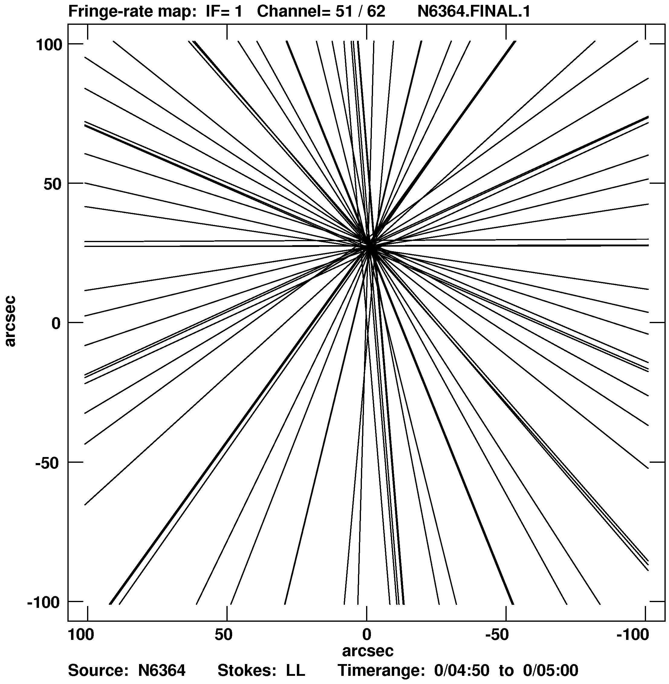
Since fringe rate is a function of source position, we can use measurements of the fringe rate to estimate the
positions of sources. Fringe rate imaging is widely used with maser sources which are usually widely separated
point objects. The angular resolution of fringe rate images is not as good as conventional aperture synthesis
imaging, but it can be used for an initial determination of the location of emitting clusters. This will help in
setting field shifts and Clean windows for use by IMAGR. Having measured the fringe rate FR(i) for
each sample in (baseline-time) and computed the derivative of fringe rate (UDOT(i)) wrt to right
ascension (X) and the derivative (V DOT(i)) wrt declination (Y ), we obtain a set of equations of straight
lines
 describing the loci of constant fringe rate for each observation. The positions of the source component(s) can be
determined by finding the places of highest density of crossing lines. (Details can be read in Giuffrida,T.S, 1977
Ph.D.thesis MIT and in Walker R.C., 1981, Astr. J., 86, 9, 1323.)
describing the loci of constant fringe rate for each observation. The positions of the source component(s) can be
determined by finding the places of highest density of crossing lines. (Details can be read in Giuffrida,T.S, 1977
Ph.D.thesis MIT and in Walker R.C., 1981, Astr. J., 86, 9, 1323.)
This algorithm is implemented in as the task FRMAP. The task plots the straight lines on the TV or prepares a
plot file. Then it determines the positions of higher density of crossing lines. The coordinates in RA and DEC of the
components found are written in an output file. The fringe rate method is especially attractive in SVLBI because of
the better angular resolution due to faster movement of the orbiting antenna. Figure 9.3 shows an example of a
fringe rate image.
FRMAP can be used for more accurate definition of the source coordinates that is required by the correlator. In
this case the correlator carries out two passes. After the first one (short) FRMAP is used to find a more
accurate position of the source. The new coordinates are then used in the second pass covering the whole
experiment.