A.2 Basic calibration

 Memo No. 76 Updated

The Gentle User enters the Computer room with a VLA archive tape containing a scientific breakthrough. The user’s sources are named source1 and source2. The interferometer phase is calibrated by observations of cal1 and cal2. The flux density scale is calibrated by observing 3C48 (=0137+331) and polarization is calibrated with observations of 3C286 and/or 3C138. Mount the tape on drive number n, log in and start . Example input: AIPS NEW. Mount the tape: INTAPE=n; DENS=6250; MOUNT.

PRTTP Find out what is on the tape, get project number and bands.  TASK=’PRTTP’; PRTLEV=-2; NFILES=0; INP; GO; WAIT; REWIND.

FILLM Load your data from tape. Select only one band at a time to process. TASK=’FILLM’; VLAOBS=’?’; BAND=’ ’; NFILES=?; DOWEIGHT 1; INP; GO (Replace all ?’s with appropriate values.) FILLM will load your visibilities (uv-data) with weights suitable for calibration into a large file for each band. It also creates 6  tables each; these tables have two letter names which are:

HI Human readable history of things done to your data. Use PRTHI to read it.

AN Antenna location and polarization tables. Antenna polarization calibration is placed here.

NX Index into visibility file based source name and observation time. Not modified by calibration.

SU Source table contains the list of sources observed and indexes into the frequency table. The flux densities of the calibration sources are entered into this table.

FQ Frequencies of observation and bandwidth with index into visibility data. Not modified.

CL Calibration table describing the antenna based gains. Version 1 should never be modified. The CL table contains entries at regular time intervals (i.e., 2 minutes) for each antenna. The ultimate goal of calibration is to create a good CL version 2. Use PRTAB to read tables.

PRTAN Print out the antenna locations. TASK=’PRTAN’; PRTLEV=0; INP; GO. Choose a good Reference antenna (called R) near the center of the array (REFANT=R). Check the VLA operator log to make sure the antenna was OK during the entire observation.

QUACK Flag the bad points at the beginning of each scan, even the ones with good amplitudes could have bad phases. Creates a Flag Table (FG). You want to use FG table version 1 for all tasks. TASK=’QUACK’; FLAGV=1; OPCOD=’ ’; APARM=0; SOUR=’ ’; INP; GO deletes the first six seconds of each scan, which may not be enough.

FG A flag table marks bad data. FG tables contain an index into the UV data based on time range, antenna number, frequency and IF number.

LISTR Lists your UV data in a variety of ways. Make a list of your observations. TASK=’LISTR’; OPTYP=’SCAN’; DOCRT=-1; SOUR=’ ’; CALC=’*’; TIMER=0; INP; GO. NOTE: IF you have observed in a way as to create more than one FREQID, you must run through the entire calibration once for EACH FREQID. For new users, it is better to use UVCOP to copy each FREQID into separate files and calibrate each file separately. This is required if you are doing polarization calibration.

UVCOP Skip this step if your data consists of only one FREQID. Copy different FREQIDs into separate files. TASK=’UVCOP’; FREQID=?; CLRON; OUTDI=INDI; INP; GO. The result will be a ??.UVCOP  file.

SETJY Sets the flux of your flux calibration source in the SU table. TASK=’SETJY’; SOUR=’3C48’,’ ’; OPTYP=’CALC’; FREQID=1; INP; GO. Adjust flux density for partial resolution following the rules in the VLA Calibration Source Manual or the  ookook.

TASAV As insurance, make a copy of all your tables. TASK=’TASAV’; CLRON; OUTDI=INDI; INP; GO.

---

Figure A.1: (left) Un-calibrated uv-data and (right) calibrated uv-data from a C-band snapshot of 3C48. Default VLA gains are a tenth of the actual gains and can show significant scatter. Only wild uv points ~50% greater than the average can be detected before calibration.

---

CALIB CALIB is the heart of the  calibration package. RUN VLAPROCS, an  runfile, to create procedures VLACALIB, VLACLCAL and VLARESET. The procedure VLACALIB runs CALIB. Set UVRANGE and ANTENNA to zero to allow use of models for 3C48. For L, C and X band 5% and 5 degree errors are OK; for other bands the limits are higher. CALIB places antenna amplitude and phase corrections into an SN table for the time of observation of phase calibration sources.

SN Solution table contains antenna based amplitude and phase corrections for the time of observations of the calibration sources. These SN table results are latter interpolated for all times of observation and placed in a CL table. Only the CL table corrections will be applied to the program sources.

TASK=’VLACAL’;  CALS=’3C48’,’ ’;  CALCODE=’*’;  REFANT=R;  UVRA=0; SNVER=1; DOCALIB=-1; DOPRINT=1;  MINAMP=10; MINPH=10; INP; VLACAL. VLACALIB will load and use a source model for 3C48, making UVRANGE unnecessary. The task CALIB lists antenna pairs which deviate significantly from the solution. If you have lots of errors, then carefully examine your data using TVFLG or LISTR. (See  ookook  for a lengthy discussion on flagging.)  If one antenna is bad over a limited time range, use UVFLG to flag that antenna for the time from just after the previous good cal observation to before the next good cal observation.

UVFLG Flag bad UV-data. TASK=’UVFLG’; ANTEN=?,0; BASELI=?,0; TIMER=?; OUTFGVER=1; SOUR=’ ’; OPCOD=’ ’; INP; GO.  If in doubt about any data, FLAG THEM! If you have flagged the primary calibrator, return to CALIB above and try again.

CALIB Now calibrate the antenna gain based on the rest of the cal sources. Look in the Calibrator manual for UV limits; if there are limits, VLACAL must be run separately for these sources. TGET VLACAL; CALS=’cal1’,’cal2’,’ ’; ANTEN=0; BASELI=0; UVRANGE=?,?; INP; VLACAL. Flag bad antennas listed. Each execution of CALIB replaces previous corrections in the SN table or appends new corrections. If unsatisfied with a VLACAL execution, all effects of it are removed by running VLACAL again for the same sources (but different ADVERBS or after flagging bad data).

GETJY Sets the flux of phase calibration sources in the SU table. TASK ’GETJY’; SOUR=’cal1,’cal2’,’ ’;  CALS=’3C48’,’ ’; BIF=0; EIF=0; INP; GO.  GETJY over-writes existing SU table entries, and is not affected by previous executions.

TASAV Good time to save your tables. TGET TASAV; INP; GO. 

CLCAL Read the antenna amplitude and phase corrections from the SN table and interpolate the corrections into a new CL table. CLCAL applies calibration source corrections to the program sources. Each execution of CLCAL adds to output CL table version 2. CLCAL is run using the procedure VLACLCAL.  TASK=’VLACLC’;  SOUR=’source1’,’cal1’,’ ’;  CALS=’cal1’,’ ’; OPCODE=’CALI’;  TIMER=0;  INTERP=’2PT’;  INP; VLACLC.  Run CLCAL for the second source using the second calibrator. TGET VLACLC; SOUR=’source2’,’cal2’,’ ’; CALS=’cal2’,’ ’; INP; VLACLC.  Move the SN table corrections for 3C48 into the CL table. TGET VLACLC; SOUR=’3C48’,’ ’;CALS=’3C48’,’ ’; INP; VLACLC. (3C48 could also be calibrated with cal1 or cal2.)

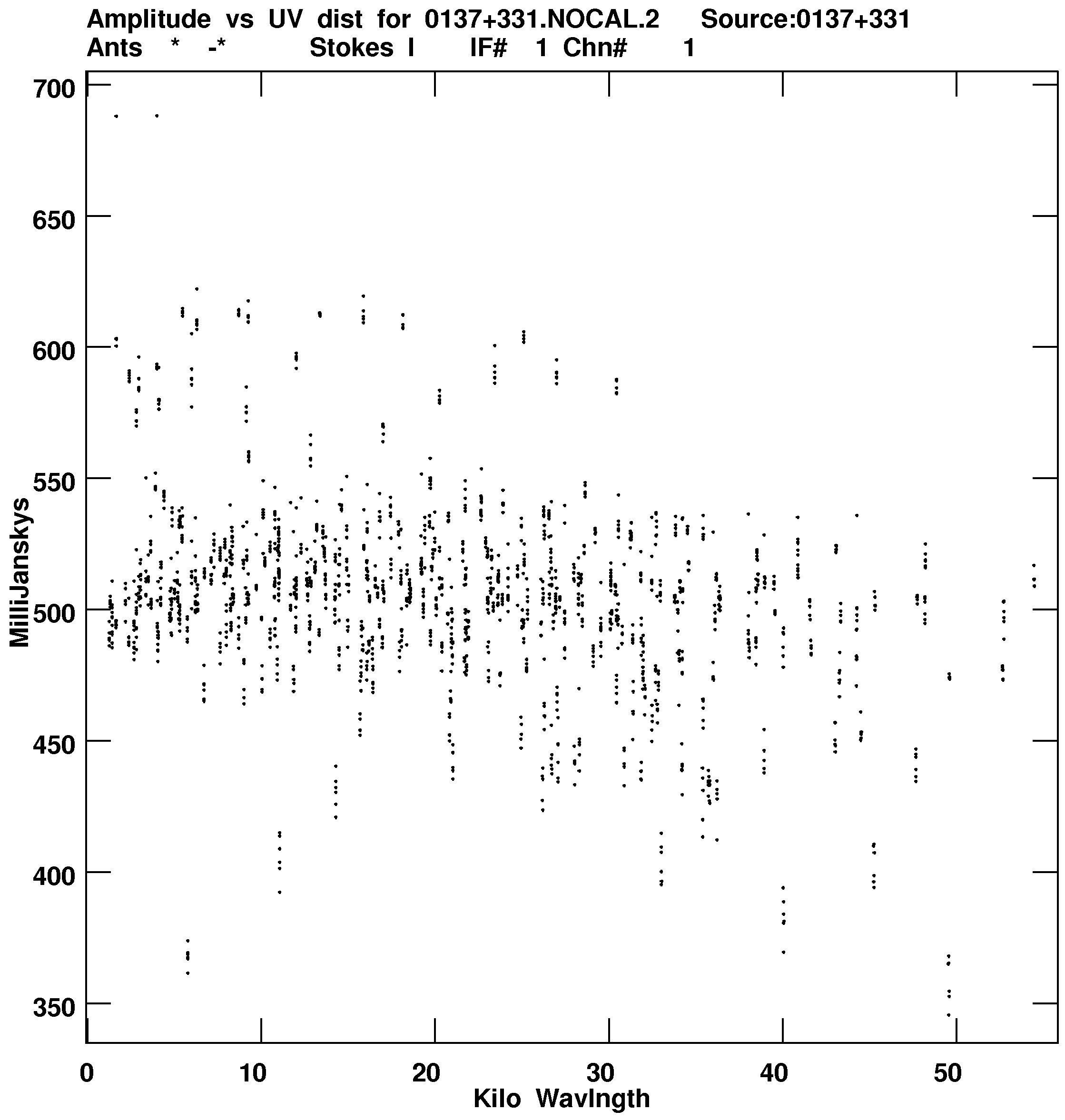
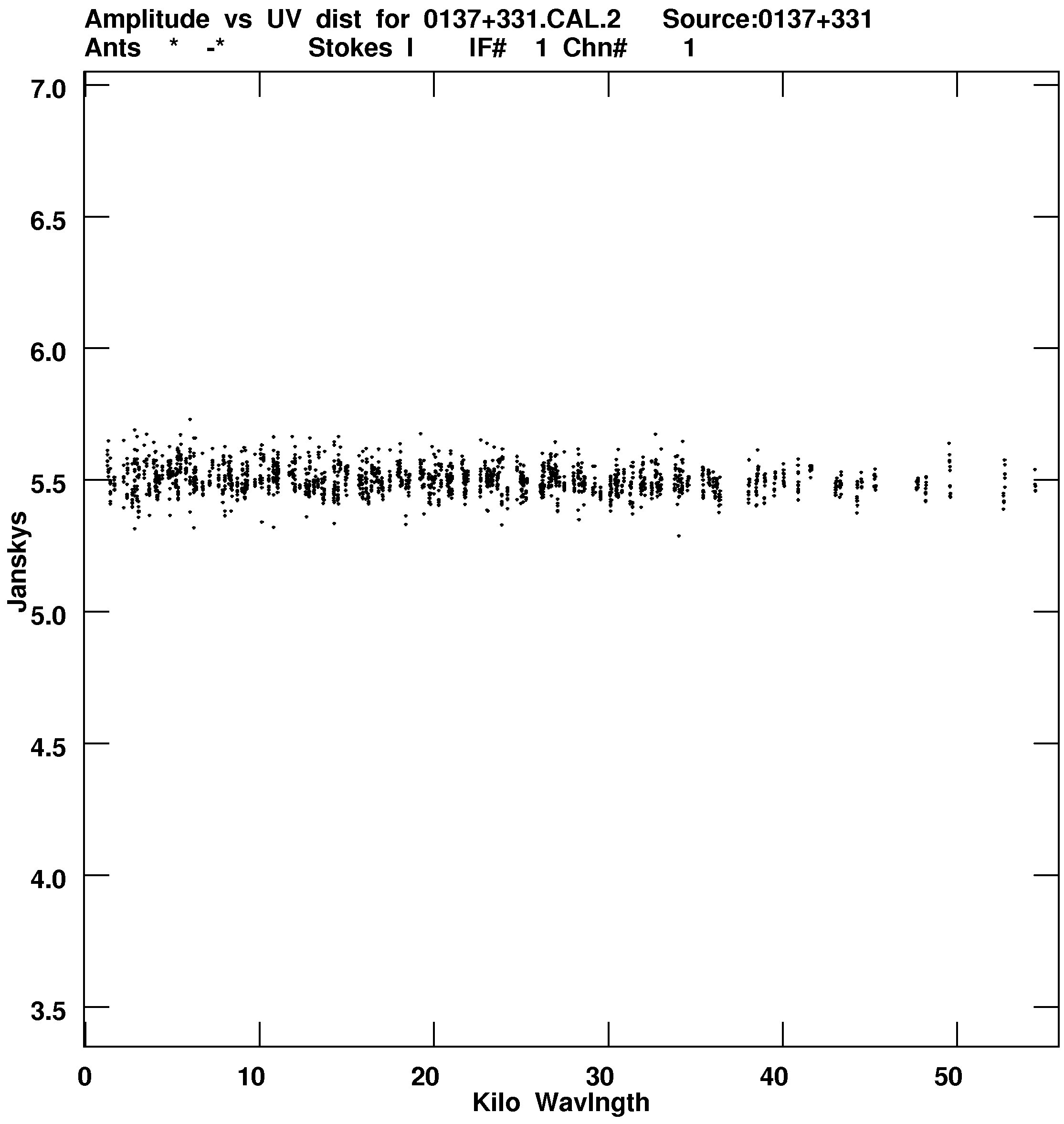
LISTR Make a matrix listing of the Amplitude and RMS of calibration sources with calibration applied. Look for wild points.  TASK=’LISTR’; OPTYP=’MATX’; SOUR=’cal1’,’cal2’,’ ’; DOCAL=2;  DOCRT=-1; DPARM=3,1,0; UVRA=0; ANTEN=0; BASELI=0; BIF=1; INP; GO.  If only a few points are bad, flag them and continue. If too many are bad, delete CL table 2 and the SN tables using VLARESET. Then return to the first CALIB step. If the data look good, run LISTR again for IF two. TGET LISTR; BIF=2; INP; GO

UVPLT Plot the uv-data in a variety of ways. Make a Flux versus Time plot first. Choose XINC so the plot will have no more than 1000 points. TASK=’UVPLT’; SOUR=’source1’,’ ’; XINC=10; BPARM(1)=11; DOCAL=2; BIF=1; INP; GO.  Look at the plot with LWPLA, TKPL, TVPL or TXPL.   Plot other IF . Flag wild points. Plot Flux versus baseline. TGET UVPLT; BPARM=0; INP; GO.

Calibration is now complete for continuum, un-polarized observations. Write the calibrated data to tape with FITTP if you don’t want to calibrate the polarization. To create images from the uv-data use SPLIT to calibrate the multi-source data and create a single source uv-data set. (FITTP and SPLIT are described at the end of the polarization calibration process.)