


 had several imaging tasks, each with distinctive capabilities, BUT they have all been superseded by IMAGR.
The abilities of IMAGR include:
had several imaging tasks, each with distinctive capabilities, BUT they have all been superseded by IMAGR.
The abilities of IMAGR include:
had several imaging tasks, each with distinctive capabilities, BUT they have all been superseded by IMAGR.
The abilities of IMAGR include:
This section will concentrate on how to use IMAGR to weight, grid, and Fourier transform the visibility data, making a “dirty beam” and a “dirty map.” We will begin with a simple example and then discuss a number of matters of image-making strategy to help make better images. Deconvolution will be discussed in the next section. This separation reflects our belief that you should first use IMAGR to explore your data to make sure that there are no gross surprises — emission from unexpected locations, “stripes” from bad calibration or interference, and the like. If you begin Cleaning immediately, you may find that you are using Clean to convert noise and sidelobes into sources while failing to image the real sources, if any. It is a good idea to make the first images of your field at the lowest resolution (heaviest taper) justified by your data. This will allow you to choose input parameters to combine imaging and Cleaning steps optimally.
We do not discuss imaging theory and strategy in much detail here because it is discussed fully in numerous lectures in Synthesis Imaging in Radio Astronomy1 .
The most basic use of IMAGR is to make an image of a single field from either a single-source data set or, applying the calibration, from a multi-source data set. Do not be discouraged by the length of the INPUTS list for IMAGR. They boil down to separate sets for calibration (with which you are familiar from Chapter 4), for basic imaging, for multi-field imaging, and for Cleaning. We will consider the second set here, the third in the next sub-section, and the last in §5.3. A standard procedure MAPPR provides a simplified access to IMAGR when calibration, polarization, multiple fields, and other more complicated options are not needed.
A typical use of IMAGR at this stage is to construct an unpolarized (Stokes I) image at low resolution and wide field to search for regions of emission or at full resolution for deconvolution by image-plane techniques discussed in §5.3.7. The following example assumes the use of an already calibrated, single-source data set:
to set the “task” name and set all IMAGR’s adverbs to initial values. |
> INP C R | to see what parameters should be set. |
> IMSIZE 1024 C R | to make a square image 1024 pixels on each side. |
> CELLSIZ 1 C R | for 1 arc-second cells. |
> UVTAP utap vtap C R | to specify the widths to 30% of the Gaussian taper in u and v in kλ (kilo-wavelengths). |
Other inputs are defaulted sensibly, which is why we started with a DEFAULT and are using the MAPPR procedure. In particular, Clean is turned off with NITER = 0, other calibrations are turned off, and all of the data (all IFs, channels, sub-arrays) will be used. Data weighting will be somewhere between pure “uniform” and pure “natural” (see §5.2.3). Note that task SETFC can be requested to examine your data file and make recommendations on the best combination of CELLSIZE and IMSIZE. Consider also both:
> HELP xxx C R |
|
where xxx is a parameter name, e.g., IMSIZE, UVWTFN, etc., to get useful information on the specific parameter. The default uv convolution function is a spheroidal function (XTYPE, YTYPE = 5) that suppresses aliasing well. Check that you are satisfied with the inputs by:
> INP C R |
|
then:
In IMAGR, you may limit the data used to an annulus in the uv plane with UVRANGE, given in kilo-wavelengths. This is a useful option in some cases, but, since it introduces a sharp edge into the data sampling and otherwise discards data that could be improving the signal-to-noise, it should be used with caution and is not available in MAPPR. Taper and other data weighting options may accomplish much the same things, but do not introduce sharp edges and do not entirely discard the data.
In the example above, we chose to make the image and each cell square. This is not required. Images can be any power of two from 64 to 16384, e.g., 2048 by 512 or 128 by 8192, if you want, and the cells may also be rectangular in arc-seconds. There may be good reasons for such choices, such as to avoid imaging blank sky (saving disk, time …) and to make the synthesized beam be roughly round when measured in pixels. Rectangularity may complicate rotating the image later with e.g., LGEOM, but the problem can be handled with the more complex HGEOM. IMAGR has the ROTATE adverb to allow you to rotate your image with respect to the usual right ascension and declination axes to align elongated source structure with the larger axis of your image.
IMAGR will create both “dirty” beam and map images. The monitor provides some important messages
while IMAGR is running. When you see IMAGRn: APPEARS TO END SUCCESSFULLY on this monitor, you should find
the requested images in your catalog using:
This would produce a listing such as:
Note that the default beam class is IBM001; the default image class will be IIM001. The images produced with NITER = 0 by IMAGR can be deconvolved by various image-plane methods (§5.3.7).
There is little real need for the multi-field capability of IMAGR unless you are Cleaning. In that case, the ability to remove components found in each field from the uv data and, thereby, to remove their sidelobes from every field, is practically a necessity. Nonetheless, it may be more efficient to make multiple fields in one GO and a good idea to check the field size and shift parameters while looking for emission sources before investing significant resources in a lengthy Clean. Task SETFC can recommend cell size, image size, and field locations to cover the central portion of the single-dish beam. In 31DEC25, adverb DOINVERS may be used to obtain an alternate set of field locations. Tasks CHKFC and FLATN may then be used to choose whichever is better for your imaging.
You specify the multiple-field information with:
> NFIELD n C R | to make images of n fields. |
> IMSIZE i,j C R | to set the minimum image size in x and y to i and j, where i and j must be integer powers of two from 64 to 8192. |
> FLDSIZ i1,j1,i2,j2,i3,j3,… C R | to set the area of interest in x and y for each field in turn. Each in and jn is rounded up to the greater of the next power of 2 and the corresponding IMSIZE. FLDSIZE controls the actual size of each image and sets an initial guess for the area over which Clean searches for components. (That area is then modified by the various box options discussed later.) |
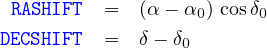
> RASHIFT x1,x2,x3,… C R | to specify the x shift of each field center from the tangent point; xn > 0 shifts the field center to the East (left). |
> DECSHIFT y1,y2,y3,… C R | to specify the y shift of each field center from the tangent point; yn > 0 shifts the field center to the North (up). |
to specify that the (u,v,w) coordinates are re-projected to the center of each field. DO3DIMAG FALSE also re-projects (u,v,w) to correct for the sky curvature while keeping all fields on the same tangent plane. The two choices now produce very similar results. |
If ROTATE is not zero, the shifts are actually with respect to the rotated coordinates, not right ascension and declination. There may be good reasons to have the fields overlap, but this can cause some problems which will be discussed in §5.3. IMAGR has an optional BOXFILE text file which may be used to specify some or all of the FLDSIZE, RASHIFT, and DECSHIFT values. To simplify the coordinate computations, the shift parameters may also be given as right ascension and declination of the field center, leaving IMAGR to compute the correct shifts, including any rotation. BOXFILE may also be used to specify initial Clean boxes for some or all fields, values for BCOMP, spectral-channel-dependent weights, and even a list of facets to ignore totally.
The OUTCLASS of the fields is controlled by IMAGR with no user assistance. For dirty images it is IIM001 for the first field, IIM002 for the second, and so forth. The I is replaced by Q, U, et al. for polarized images and the IM is replaced by CL when Cleaning. When ONEBEAM is true, one beam of class IBM001 is used for all fields. When ONEBEAM is false, a beam of class IBMnnn is used for fields of class IIMnnn or ICLnnn, with similar substitutions for other Stokes parameters.
Users are often confused by the fact that radio synthesis images are made in a rectangular coordinate system of
direction cosines that represents a projection of angular coordinates onto a tangent plane. Over wide fields of view,
the image coordinates are not simple scalings of right ascension and declination. For details of all coordinate
systems supported by , please consult Memos No. 27, “Nonlinear Coordinate Systems in ,”
and No. 46, “Additional Non-linear Coordinates,” by E. W. Greisen (available via the World-Wide Web §3.8 and
§3.10.3).2
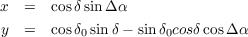
The coordinate system for VLA images is the SIN projection, for which the image coordinates x and y relate to right
ascension α and declination δ as
For many practical purposes, it is sufficiently accurate to suppose that imaging parameters do correspond to simple
angular shifts of the image on the sky. input terminology reflects this simplification, although actual coordinate
shifts and transformations in all tasks and verbs are accomplished rigorously using the full non-linear
expressions. If you want to relate shifts in pixels (image cells) to shifts in sky coordinates (α, δ) manually, you
must understand, and take account of, the non-linear coordinate system yourself. The verb IMVAL can
help by displaying the non-linear coordinates for the specified input pixel. This is rarely necessary,
however.
The minimum noise in an image is produced by weighting each sample by the inverse square of its uncertainty
(thermal noise). assumes that the input weights are of this form, namely W ∝ 1∕σ2. FILLM offers the option,
for VLA data, of weighting data in this fashion using recorded system temperatures (actually “nominal
sensitivities”). EVLA data may be weighted using SysPower data with TYAPL or simply with the variances found in
the data with REWAY. Channel-dependent weights may also be determined by BPWAY which finds a normalized
weighting “bandpass.” The resulting weights are reasonably accurate for this use after calibration. In some cases,
weights are simply based on integration times and the assumption that each antenna in the array had the same
system temperature. If the weights are not of the correct form, run REWAY or, if necessary,FIXWT on the uv data set to
calculate weights based on the variances in the data themselves. Then to get the minimum-noise image,
specify
> UVWTFN ’NA’ C R | to get “natural” weighting. |
to have all samples simply weighted by their input weights. Unfortunately, most interferometers do not sample the uv plane at all uniformly. Typically, they produce large numbers of samples at short spacings with clumps of samples and of holes at longer spacings. Thus, the beam pattern produced by natural weighting tends to have a central beam resembling a core-halo source with the broad halo (or plateau) produced by all the short spacing data and also to have rather large sidelobes due to the clumps and holes. In some VLBI arrays, data from some baselines have weights much much greater than from other baselines due to differences in antenna size and receiver temperature. Only the high-weight baselines contribute significantly to a natural-weighted image in this case.
To reduce the effects of non-uniformity in data sampling, the concept of “uniform” weighting was devised. In its purest form, uniform weighting attempts to give each cell in the uv-plane grid the same weight. Thus, the weight given each sample, is its weight divided by the sum of weights of all samples in the cell in which it occurs. In this case, in some cells a sample will count at full weight while in another, possibly adjacent, cell a sample will count at only a small fraction of its weight. To obtain this classic weighting in IMAGR enter:
to specify a weight grid the size of the image grid and the default weighting scheme. |
> ROBUST = -7 C R | to turn off all weight tempering. |
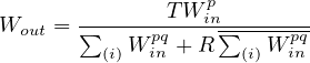
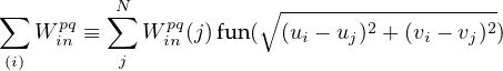
IMAGR actually implements a far more flexible (and therefore more complicated) scheme to give you a wide range of weighting choices. The intent of uniform weighting is to weight a sample inversely with respect to the local density of data weights in a wider sense than the default cell boundaries. IMAGR allows you to choose the size of cells in the uv plane with UVSIZE, the radius in units of these cells over which each sample is counted with UVBOX, and the way in which each sample is counted over this radius with UVBXFN. The weighting grid can be smaller or larger than the image grid. You can even make the uv cells be very small by specifying a very large UVSIZE; you are limited only by the available memory in your computer and the time you wish to spend weighting the data. Note, of course, that uniform and natural weighting are the same if the cells are small enough unless you specify a significant radius over which to count the samples. IMAGR does not stop here, however. It also allows you to alter the weights before they are used, to count samples rather than weights, and to temper the uniform weights with Dan Briggs’ “robustness” parameter. Thus
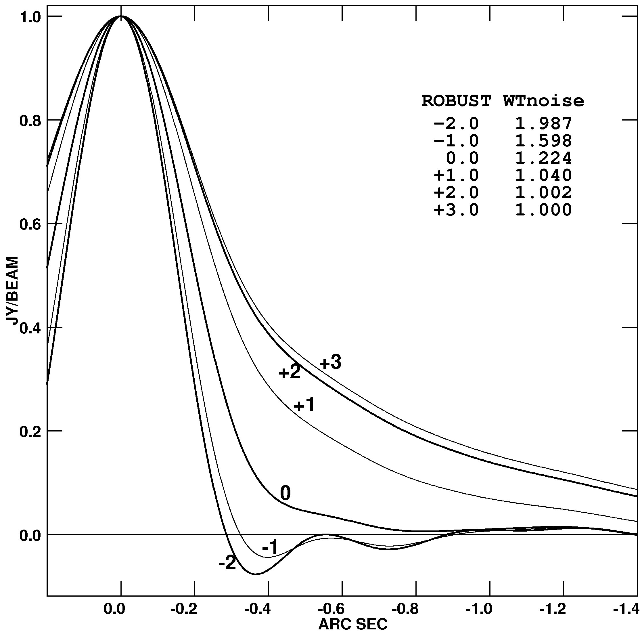
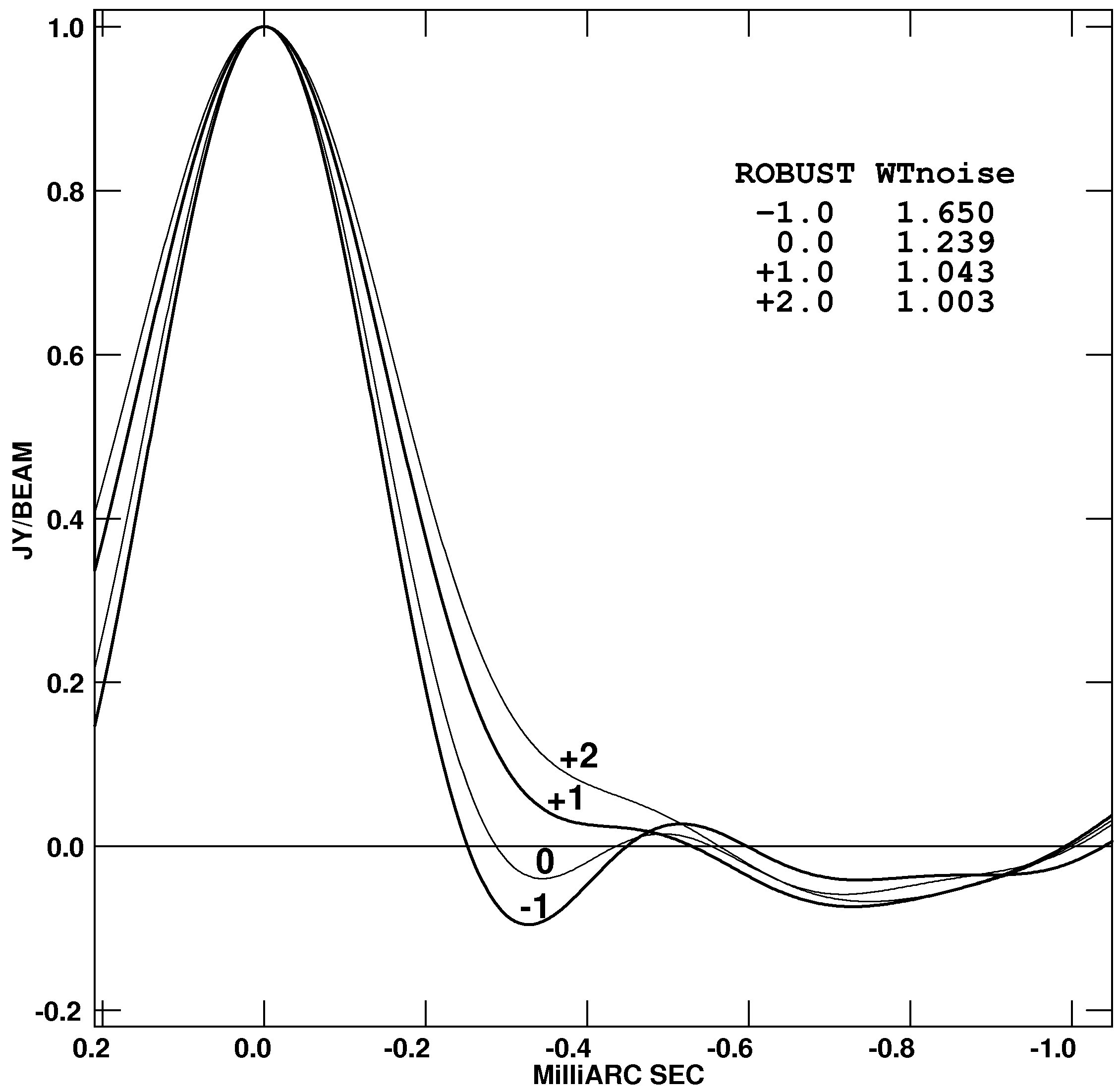
At this point you should be totally confused. To some extent, we are. While IMAGR has been around for a while, the impact of all of these parameters on imaging is not well understood. You may wish to experiment since it is known — see figures on next page — that weighting can make a significant difference in the signal-to-noise on images, can alter the synthesized beam width and sidelobe pattern, and can produce bad striping in the data when mildly wrong samples get substantially large weights. The default values do seem to produce desirable results, fortunately. The beam width is nearly as narrow as that of pure uniform weighting, but the near-in sidelobes are neither the positive “shelf” of pure natural weighting nor the deep negative sidelobes of pure uniform weighting. The expected noise in the image is usually rather better than for pure uniform weighting and sometimes approaches that of natural weighting. Deconvolution should be improved with reduction of erroneous stripes, noise, and sidelobe levels. You should explore a range of UVTAPER and ROBUST (at least) in a systematic way in order to make an informed choice of parameters.
The option to average the input data in time over a baseline-length dependent interval adds further complications. It has the desirable effect of reducing the size of your work file, thereby speeding the imaging process. But it changes the distribution of data samples ahead of uniform weighting since it averages the short-spacing samples a great deal more than the long-spacing samples. This makes natural weighting less undesirable and causes uniform weighting to be less sensitive to extended source structures. Set IM2PARM(11) and (12) to request this option. IM2PARM(13) adds frequency averaging to the time averaging option. It may be desirable to keep narrow spectral channels in the data set for editing purposes, but the bandwidth synthesis may be speeded up significant while causing no degradation by a judicious choice of channel averaging.
If your source has complicated fine structure and has been observed with the VLA at declinations south of about +50∘, there may be important visibility structure in the outer regions of the uv plane that is sampled sparsely, even by “full synthesis” imaging. In such cases, Clean may give images of higher dynamic range if you are not too greedy for resolution at the imaging stage. Use UVTAPER to down-weight the poorly sampled outer segments of the uv plane in such cases. (UVRANGE could be used to exclude these data, but that introduces a sharp discontinuity in the data sampling with a consequent increase in sidelobe levels.) Tapering is, to some extent, a smooth inverse of uniform weighting; it down-weights longer spacings while uniform weighting down-weights shorter spacings in most arrays. The combination can produce an approximation to natural weighting that is smooth spatially.
IMAGR does all weighting, including tapering, in one place and reports the loss in signal-to-noise ratio from natural weighting due to the combination of weighting functions. This reported number does not include the loss due to discarding data via UVRANGE, GUARD, the finite size of the uv-plane grid, data editing, and the like.
Other things being equal, the accuracy of beam deconvolution algorithms (§5.3) generally improves when the shape of the dirty beam is well sampled. When imaging complicated fields, it may be necessary to compromise between cell size and field of view, however. If you are going to Clean an image, you should set your imaging parameters so that there will be at least three or four cells across the main lobe of the dirty beam.
Actually, this is not the full story. If you have a large number of samples toward the outer portions of the uv-data grid, then the width of the main lobe of the dirty beam will not be correctly measured. Making the cell size smaller — raising the size of the uv-data grid (in wavelengths) — will change the apparent beam width even if no additional data samples are included. Even when you have a cell size small enough to accurately represent the dirty beam, the presence of samples in the outer portion of the uv-data grid can confuse high dynamic-range deconvolution. The high-resolution information contained in these outer samples cannot be represented with point sources separated by integer numbers of too-large cells. The result is a sine wave of plus and minus intensities, usually in the x or y direction, radiating away from bright point objects and a Clean that always finds a component of opposite sign at a virtually adjacent pixel whenever a component is taken at the bright point sources. This is often a subtle effect lost in the welter of long Cleans, but has led to the concept of a “guard” band in the uv-data grid. The adverb GUARD in IMAGR and friends, controls the portion of the outer uv-data grid which is kept empty forcibly by omitting any data that would appear there. The default is the outer 30% of the radius (or less if there is taper), which is a compromise between the 50% that it probably should be and the epsilon that some vocal individuals believe is correct. All imaging tasks will tell you if they omit data because they fall off the grid or outside the guard band and will warn you of possible Cleaning problems if data lie inside the guard band but outside a more conservative guard band.
Because Clean attempts to represent the brightness distribution of your source as an array of δ-functions, the deconvolution will have higher dynamic range if the brightest point-like features in your images have their maxima exactly at pixel locations. In this case, the brightest features can be well represented by δ-functions located at image grid points. If you are pursuing high dynamic range, it may therefore be worth adjusting the image shift and cell-size parameters so that the peaks of the two brightest point-like features in your image lie exactly on pixels.
If you are going to use image-plane deconvolutions such as APCLN, SDCLN, or VTESS, you must image a large enough field that no strong sources whose sidelobes will affect your image have been aliased by the FFT and so that all real emission is contained within the central quarter of the image area. With IMAGR, you should make a small image field around each confusing source (or use Clean boxes within larger fields).
You help Clean to guess what may have happened in the unsampled “hole” at the center of the uv plane by including a zero-spacing (usually single-dish) flux density when you make the image. This gives Clean a datum to “aim at” in the center of the uv plane. Extended structure can often be reconstructed by deep Cleaning when the zero-spacing flux density is between 100% and ~125% of the average visibility amplitude at the shortest spacings (run UVPLT to estimate this average for your data set). If your data do not meet this criterion, there may be no reliable way for you to image the extended structure of your source without adding further information to your observations (e.g., by adding uv data from a more compact array, by Fourier transforming a suitably tapered and deconvolved single dish image of the VLA primary beam, or by using such an image as the default image for a maximum entropy deconvolution as in §5.3.7). See §10.5 for further discussion. IMAGR treats the zero spacing differently from previous tasks. The adverb ZEROSP gives five values, the I, Q, U, V fluxes, and a weight. This weight should be in the same units as for your other data, since the ZEROSP sample is simply appended to your data set and re-weighted and gridded just like any other data sample. To have the zero spacing be used, both ZEROSP(1) and ZEROSP(5) must be greater than zero, even when you are imaging some other polarization. Previous “wisdom” held that the weight should be “the number of cells that are empty in the center of the uv plane,” but this does not appear to be correct with IMAGR.
If UVPLT shows a rapid increase in visibility amplitudes on the few shortest baselines in your data, but not to a value near the integrated flux density in your field, you may get better images of the fine structure in your source by excluding these short baselines with the UVRANGE parameter. There is no way to reconstruct the large-scale structure of your source if you did not observe it, and the few remnants of that structure in your data set may just confuse the deconvolution. Be aware that, in this circumstance, you cannot require your image of total intensity to be everywhere positive. The fine-scale structure can consist of both positive and negative variations on the underlying large-scale structure.