D.1 Complications at higher frequencies

High-frequency data (22 or 43 GHz) from the VLA may be reduced occasionally with the standard centimeter-wavelength recipe given in this ookook, particularly in the smaller arrays. However, quire frequently,, the standard recipe will be inadequate for such data, particularly in the larger (A and B) array configurations. Nevertheless, VLA data taken at these high-frequencies in the largest array configurations can be calibrated in almost all cases with only a few minor adjustments to the centimeter wavelength recipe.

One reason for more complicated calibration is the high resolution, which resolves the standard flux density calibrators, particularly 3C48. However, most of the problems are caused by the atmosphere, where the troposphere introduces rapid phase fluctuations between the antenna elements of the interferometer. Both effects scale with baseline length expressed in units of wavelength, but the latter also heavily depends on the current weather; phases are sometimes observed to wind on time scales of less than a minute. This causes decorrelation during your calibrator and target source scans, and requires you to determine phase-only calibration, before the flux density (i.e., gain) calibration should be attempted.

In this appendix, an approach to reducing high-frequency VLA data in  is described which should help to overcome the most common problems. It is assumed that the reader has some experience with reducing data in , and is familiar with the “standard recipe” (e.g., Appendix A), tools to examine the data, to apply self-cal, and if appropriate, to deal with spectral-line and polarization calibration issues. If not, you should read the  ookook first (in particular Chapter 4).

High-frequency calibration begins when loading the data, requiring specific parameters in FILLM to be set (ideally one should use these FILLM inputs for all frequencies).

Run FILLM with:

This creates a CL table that can be interpolated over very short intervals, hopefully short enough to cover the atmospheric phase fluctuations accurately. The default CL table interval is 5 minutes, which may be fine for centimeter wavelengths, but is much too long for proper interpolation of high-frequency phases. Also, you have “nominal sensitivity” weights for individual IF/Pol entries, which reflect sensitivity differences between the receivers, IFs, etc. To retain this “nominal sensitivity” weighting you are required to set DOCALIB=1 (actually 0 < DOCALIB ≤ 99 and a non-negative value for GAINUSE) in all the calibration tasks during the remainder of the data calibration.

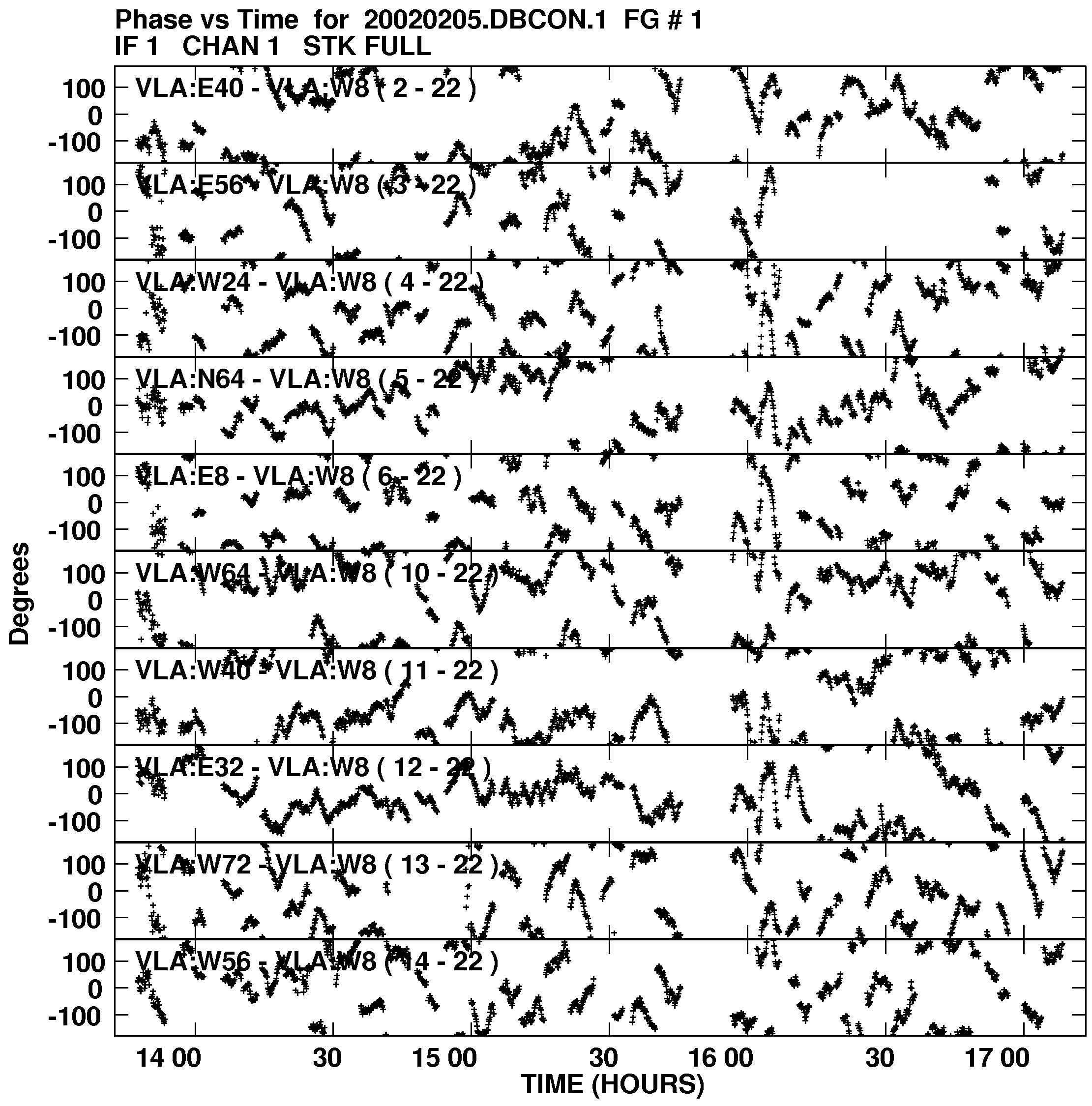
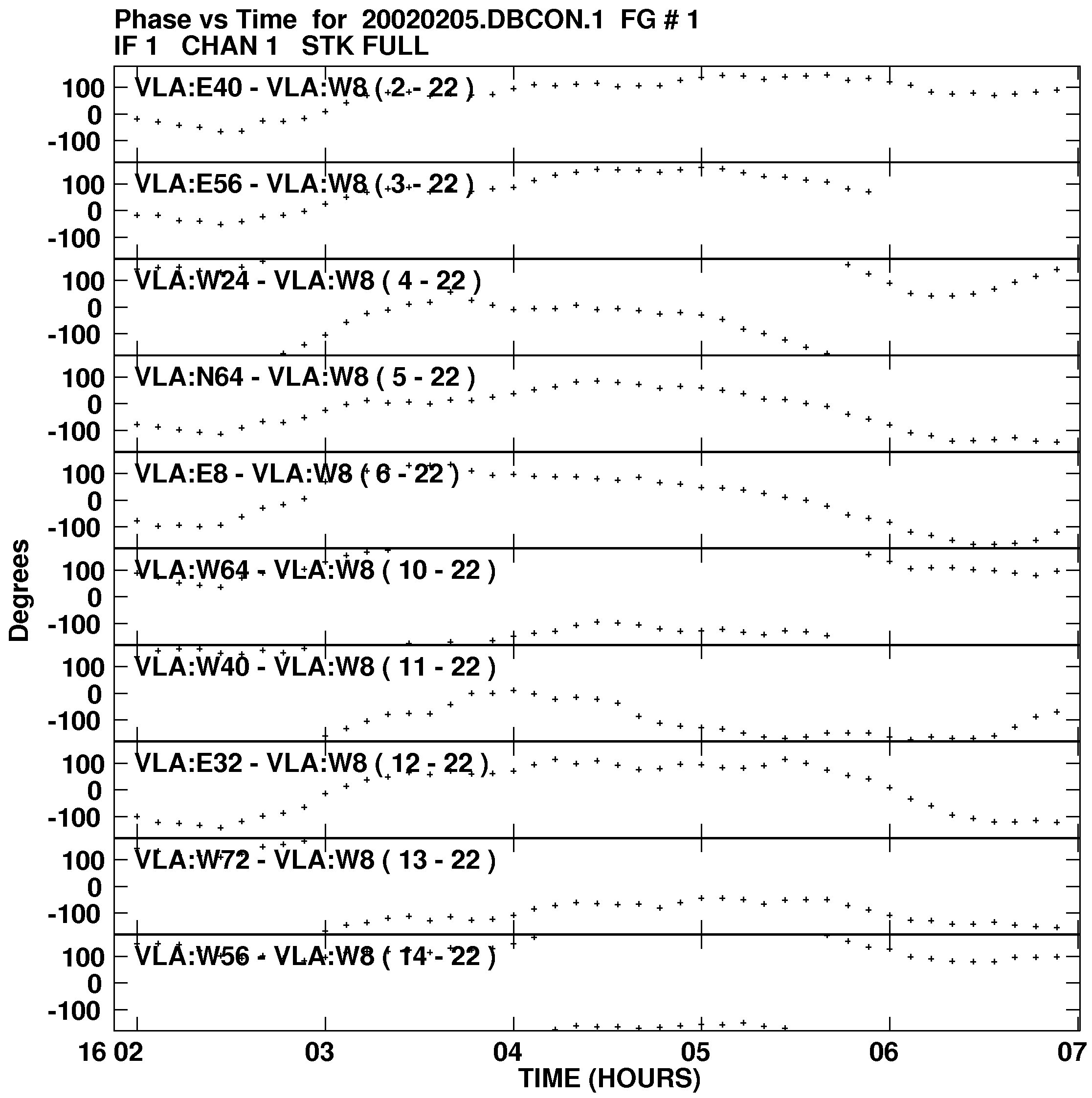
The importance of the CL table interval is illustrated in Figure D.1 and Figure D.2. On the large scale, the phases look beyond redemption. But, on a relatively short time scale, the phases are relatively well behaved and may be calibrated easily.

After loading your data, check your CL table entries, e.g., LISTR with OPTYPE ’GAIN’, PRTAB with DOHMS 1, or SNPLT on a short (few minutes) time range with OPTYPE ’AMP’. Make sure the entries are at the interval you expect (much less than a minute) and that the opacity and gain curve corrections have been applied (gains deviating from one by a few percent). Inspect your continuum or “channel 0” data (gains, system temperatures), and flag bad data. For example, you also may wish to flag antenna 1, which is known to have bad optics at 43 GHz, and the antennas without a 43 GHz receiver (currently in December 2002, antennas 9 and 15, but for earlier observations you may want to check the receiver status page (http://www.vla.nrao.edu/astro/guides/highfreq/), or your observation log — these antennas may have been left present in your data when you first do a pointing scan in X-band). Standard tools for data inspection and flagging are described in Chapter 4 of the  ookook (LISTR, UVPRT, VPLOT, SNPLT, SNBLP, UVFLG, TVFLG, EDITR, EDITA, and many more). Make sure that at least your calibrators are “clean.” Run VPLOT on your calibrators with a reference antenna close to the center of the array (determined by using PRTAN) to get an indication how rapidly your phases fluctuate; use ANTENNA reference_antenna 0; SOLINT 0; BPARM 0 2 0 (for phase only). If your program source is too weak to allow self-calibration and the phase change from one scan on your calibrator to the next is of the order of 180^∘, you probably want to flag the source data in between the calibrator scans. Task SNBLP will let you examine how the calibration affects each baseline and task SNFLG may be useful for doing this flagging.

Note that fast-switching, when used, will have changed the source names you used in making the observe schedule file. Your sources will have been renamed to their J2000 positions, making it difficult to recognize the calibrator and target scans when you run LISTR (OPTYPE ’SCAN’).

Run SETJY on your absolute flux density calibrator: 3C286 = J1331+305 = B1328+307, or 3C48 = J0137+331 = B0134+329. And maybe it is a good idea to make a copy of your correct CL table number one (actually all tables) with TASAV before continuing, so in case of accidents, you have CL table one with the opacity/gain corrections applied. (INDXR may be used to re-create a CL table, including the opacity and gain corrections made by FILLM.

Run VLANT to correct phases for improved estimates of the antenna positions. Note that this task requires your computer to be connected to the Internet if your data are recent (within past 18 months or so). Otherwise, apply baseline corrections following advice at www.vla.nrao.edu/astro/archive/baselines/.

Run CALIB, at this stage to correct for phase only, with a small solution interval (depending on your signal to noise, e.g., 20 seconds) on all your calibrator sources. You should use the Clean-components models for 3C286 or 3C48 provided with . See §4.3.9.1 for information on CALDIR and CALRD. Then run CALIB on these sources separately using the appropriate model. There are also models for 3C147 and 3C138.

Inputs to the first pass of CALIB:

And, if you have 3C48, 3C138, 3C147, and/or 3C286 as absolute flux density calibrator(s), you should re-run CALIB, one calibrator source at a time, with the previous/above values plus:

This may work, but there is no guarantee. Some tricks to apply, in no particular order, in your data set or CALIB to obtain a larger relative portion of good versus bad solutions would be:

•  Flag some more bad data points on your calibrator sources.
•  Discard antennas with uncertain baseline positions (see observing log file).
•  Choose a different reference antenna (the one you have might be misbehaving).
•  Decrease the UVRANGE to weight short baselines (centrally located antennas) more in the solution.
•  Use SOLTYPE ’L1’ to be less sensitive to outlying points.
•  Use FRING instead of CALIB with a larger SOLINT to solve for the phase rates, switching off the delay search with DPARM(2) = -1.
•  Increase or decrease SOLINT; increase for weak, decrease for strong sources.
•  Decrease the SNR cutoff APARM(7) (default 5) to include more noisy but possibly valid solutions.
•  Decrease the number of antennas required for a solution (APARM(1), default 6) to require fewer antennas
•  Recreate ’CH 0’ from ’LINE’ to get up to 25% more bandwidth on calibrators.

Note that at 43 GHz in A-array the unprojected uv-distance between the outer two antennas on one arm is 0.5 Mega-wavelengths, and the outer 6 antennas — the default for APARM(1) — require good solutions out to 2 Mega-wavelengths for CALIB to accept the solution for your outermost antenna. Hence, it is a good idea to set APARM(1) to e.g., four (or three, if you’re willing to check the output SN table carefully).

Check the resulting SN table number one with LISTR (OPTYPE ’GAIN’, DPARM 1 0) or SNPLT (INEXT ’SN’, OPTYPE ’PHAS’), and judge whether you have enough solutions and whether you believe the phases shown are likely to reflect the variation caused by the troposphere. If not, fiddle around with your data and/or parameters in CALIB as suggested above and try again. In case the majority of solutions are fine, you may want to edit spurious points in your SN table with e.g., SNEDT, SNCOR, or SNSMO.

Once you are satisfied with the phases in your SN table, you want to apply phase corrections to minimize decorrelation in your calibrator scans before you determine the absolute flux density scale. To insert the corrections, run CLCAL with:

In less straightforward observations you may not be able to run CLCAL only once, e.g., when you are switching frequencies. If in doubt, consult Chapter 4 of the  ookook. It is however very simple to run CLCAL multiple times. Inspect your new CL table two (three after VLANT) for unexpected dubious interpolations and extrapolations (LISTR with OPTYPE ’GAIN’, DPARM 1 0, or SNPLT with INEXT ’CL’, OPTYPE ’PHAS’) and backtrack possible problems. SNBLP should help you to find problem solutions as they affect your data.

Now re-run CALIB with the corrected phases to obtain the flux density scale. Begin with those sources not requiring models:

Then run CALIB again for the absolute flux density calibrator 3C286, or 3C48, using a model and the previous/above values plus:

The same tricks may be used as for phase-only to improve the ratio of good to bad solutions. Check your SN table 2 thoroughly; the phases must be zero or very close to zero (therefore INTERPOL ’2PT’ is preferred over INTERPOL ’SIMP’ in CLCAL), and you want to make sure the gains of your reference antenna do not scatter too much for individual sources. Before GETJY the flux density scale is not fixed so the average gain will depend on source. GETJY corrects this so that the gains for each antenna should be similar for all sources. If you can identify misbehaving antennas, flag them, delete SN table 2 (as it does not overwrite values for which data have been deleted), and re-run CALIB as many times as needed to re-create SN table two. Cautious users will start from the beginning.

Run GETJY to obtain the secondary calibrator flux densities:

If you used a model for the flux density calibrator, your flux scale is tied to the flux density of that calibrator in the SU table. The model Clean components are scaled to match that flux.

Carefully note the flux densities reported by GETJY and do not trust these values blindly. LISTR or SNPLT may point out problematic antenna solutions, requiring you to flag some more data and start over. If you flag data, it is best to delete SN table #2. Solutions at the times of deleted data will not be overwritten. It is helpful to know what flux you expect for your secondary calibrators. See the full source list at aips2.nrao.edu/vla/calflux.html. It is particularly helpful to use one or more of the sources regularly monitored by NRAO staff; see html://www.aoc.nrao.edu/~smyers/calibration/ for total flux as well as polarization information. You want to check the values, because sometimes the flux densities deviate considerably from the expected values and make no sense. This could be the case if the pointing solutions that were determined prior to your primary calibrator scan are inappropriate for this particular primary calibrator scan e.g., when it is windy or when the cloud cover on your single primary calibrator scan differs from the cloud cover on the secondary calibrators, or, even worse, when these combine. In some cases you may be forced to approximate the flux density scale by entering a (recent) flux density for one of your secondary calibrators, ignoring the primary calibrator scan and accepting an introduced flux density uncertainty. If you decide you have to restart, do not forget to delete your SN and CL tables (except for CL table 1 and 2 if you used VLANT) and to reset the flux densities of all your calibrators with SETJY (OPTYPE ’REJY’), before entering a ZEROSP for a new flux density calibrator source (also with SETJY). Re-iterate until you are happy with the flux-density scale.

The final flux density calibration table is obtained by running CLCAL again:

From here you are almost ready to follow the usual “standard recipe,” i.e., polarization and bandpass calibration if appropriate, and splitting into single-source data sets. However, remember to set DOCALIB = 1 in all these tasks as long as you are working on the multi-source data set and haven’t applied initial phase, flux density (including polarization, bandpass) and “nominal sensitivity” calibration with SPLIT. After SPLIT, the individual weights will have been entered in the data, properly scaled by the latest CL table you’ve made. Using your single source calibrated data, set DOCALIB = -1 in your subsequent imaging and analysis tasks, unless you do self-calibration.

If you anticipated checking your fast-switching calibration by including a “check source” (a moderately strong source observed a few times with the same fast-switching parameters at about the same distance from your fast-switching source as your target source, but not necessarily in the same direction), you can now assess a snapshot of your calibration by imaging this source. If the fast-switching has worked perfectly, your check source has the expected morphology, flux density, and position. Any position error on the check source should indicate the accuracy of the astrometry on your target source. If you did not include a check source, all but the astrometry and spatial dependence of the calibration can be inferred from your fast-switching source by imaging a scan (use a modified SN/CL table by skipping the calibration on this scan) with the calibration derived from the two neighboring scans.