
Handling EVLA data is quite different from the situation with the historic VLA. The principal difference is the very wide bandwidth of the EVLA which makes every data set have a large number of spectral channels in every spectral window. This requires corrections for delay errors and bandpass shape which were not needed with historic VLA continuum data. It also means that almost all observations are contaminated by radio frequency interference (RFI) at a level requiring that some portion of the data be marked as bad (“flagged”) and omitted from later use. Writing a general list of calibration steps is rather difficult because the steps needed depend on the problems found in the data set. Low frequency data (bands less than 8 GHz) are likely to be heavily contaminated with RFI, while the highest frequency bands have very little. But the high frequencies suffer greatly from rapidly varying “instrumental” (i.e., atmospheric) phase variation. Nonetheless, we will make a list of the general steps that need to be taken following those already described.
Sometimes, e.g., during a VLA array re-configuration, your observations may have been made when one or more of the antennas had their positions poorly determined. The positional error is usually less than a centimeter at the VLA, but even this may affect your data significantly. The most important effect is a slow and erroneous phase wind which is a function of source position and time. Since this error is a function of source position, it cannot be removed exactly using observations of a nearby calibrator, although the error will be small if the target source is close to the calibrator. In many observations, the target sources and calibrators are sufficiently close to allow this phase error to be ignored. Self-calibration will remove this error completely if you have enough signal-to-noise to determine the correction during each integration.
The maximum phase error introduced into the calibrated visibility data by incorrect antenna coordinates ΔϕB, in radians, by a baseline error of ΔB meters is given by
Note, however, that the error due to the phase-wind is not the only error introduced by incorrect antenna positions. A further, but much smaller effect, will be incorrect gridding of the data due to the erroneous calculation of the baseline spatial frequency components u, v and w. This effect is important only for full primary beam observations in which the antenna position error is of the order of a meter. It is highly unlikely that such a condition will occur. Note too, that this error cannot be corrected by the use of self-calibration. However, after correcting the antenna position with CLCOR, you may run UVFIX to compute corrected values of u,v, and w. The maximum phase error in degrees, ΔϕG, caused by incorrect gridding of the u,v,w data is

If baseline errors are significant they need to be removed from your data before calibration. It is important to do this to CL table 1, right after running BDF2AIPS. For the EVLA, use the task VLANT. This task determines and applies the antenna position corrections found by the VLA operations staff after your observation was complete. To run VLANT:
to get the correct data set. Note that you don’t have to keep doing this unless you switch between different input data files. |
> FREQID 1 C R | to choose FQ 1. |
> SUBARRAY x C R | to choose the antenna table to correct. |
> GAINVER 1 C R | to choose the correct version of the CL table to read. A new one will produced. |
For arrays other than the VLA, use CLCOR to enter the antenna position corrections (in meters) in a new CL table and the old AN table. This must be done for each affected antenna in turn. CLCOR puts the corrections into the AN table as well as the CL table, so it is wise to save the AN table before running CLCOR by running TASAV.
to get the correct data set. Note that you don’t have to keep doing this unless you switch between different input data files. |
> SUBARRAY x C R | to choose the correct sub-array. |
> OPCODE ’ANTP’ C R | to select the antenna position correction mode. |
> GAINVER 1 C R | to choose the correct version of the CL table to read. |
> ANTENNA k C R | to select antenna. |
> CLCORPRM Δbx, Δby, Δbz, 0 C R | to add the appropriate antenna corrections in meters. |
The program will need to be run as many times as there are antennas for which positional corrections must be made. Set GAINUSE and GAINVER both to 2 after the first correction. Otherwise, with the above adverbs, CLCOR will make multiple CL table versions each with only one correction in them. Note that subsequent calibration must be applied to CL table 2 to create higher versions of the calibration table. This new CL table (version 2) will replace version 1 in all of the subsequent sections on calibration. Thus, in subsequent executions of CALIB, you must apply these corrections by specifying DOCALIB TRUE ; GAINUSE 0 (for highest version). Note too that CLCOR and VLANT change the antenna file for the changed antenna location(s). Therefore, it is wise to save the AN table before running CLCOR or VLANT by running TASAV.
Note that NRAO’s data analysts use the 


 task LOCIT to determine the antenna position corrections; see
Appendix V.. These are available to the general user, but a data set designed to determine antenna corrections is
normally required. Such data sets consist of about 100 observations of a wide range of phase calibrators taken as
rapidly as possible.
task LOCIT to determine the antenna position corrections; see
Appendix V.. These are available to the general user, but a data set designed to determine antenna corrections is
normally required. Such data sets consist of about 100 observations of a wide range of phase calibrators taken as
rapidly as possible.
With the historic VLA, the system temperature was measured in real time and a correction for it applied to the data as they were archived. With the EVLA this is not the case. Instead the SY table records the total power when the switched noise tubes are on and the total power when they are off. These values may be used to correct data taken with 8-bit correlation (§4.3.15) to values which would be fully calibrated in Janskys if the noise tube levels and antenna efficiencies were accurately known. For 3-bit data, frequently used to observe very wide bandwidths at high frequency, the the function to correct the visibilities from these measurements is not well known. As a consequence, for such data, we can only correct for any post-detector gain changes. These are also recorded in the SY table, so use
> INEXT ’SY’ C R | to specify an SY table. |
> OPTYPE ’PGN’ C R | to specify the post-detector gain correction. |
> INP C R | to check the inputs. |
> GO C R | to write out a new data set with gain corrections. |
Reminder — do this only for 3-bit correlator data. Your 8-bit data will be discussed later.
The next step is to take a look at your data. Do not be obsessive about this. Choose your main calibration
source (that you plan to use for FRING, BPASS, and absolute gain calibration), choose a few baselines
(say all baselines to one interior antenna), and use the TV display. At this point you want to
look for antennas that appear out of the ordinary (i.e., dead) and for frequencies damaged by RFI.
Use
> SOURCE ’bandpass_cal’ C R | to select the strong bandpass calibrator. |
> ANTEN n1 , 0 C R | to select an antenna nearest the center of the array. |
> BASELINE 0 C R | and all antennas to that antenna. |
to apply the initial calibrations and display vector averaged spectra. Scalar averaged spectra will turn up at the edges reflecting the decreased signal to noise in the outer channels. |
> APARM(9)=3 C R | to plot all IFs and both polarizations in a single plot. |
> GO C R | to run the task. Make notes of what you see. |
If there is very narrow-band RFI, the POSSM plots will show ringing - a sin(x)∕x pattern as a function of spectral channel. If this occurs in your data, and it will not occur in some bands, then
> SMOOTH 1,0 C R | to use Hanning smoothing. |
> INP C R | always check the many inputs which should be defaults here. |
> GO C R | to make a new data set with the ringing reduced. |
At this point, it is essential only to flag the most egregiously bad data samples. These are, with the EVLA, usually either dead antennas or spectral regions affected more or less uniformly by RFI. We will however use this section for a more general discussion of flagging, most of which will apply more directly to later stages in the reduction. Probably FTFLG may be used carefully at this stage to flag only those channels seen to be generally bad in the POSSM plots.
The philosophy of editing and the choice of methods are matters of personal taste and the advice given below should, therefore, be taken with a few grains of salt. When interferometers consisted of only a couple of movable antennas, there was very little data and it was sparsely sampled. At that time, careful editing to delete all suspect samples, but to preserve all samples which can be calibrated, was probably justified. But modern instruments produce a flood of data, with the substantial redundancy that allows for self-calibration on strong sources. Devoting the same care today to editing is therefore very expensive in your time, while the loss of data needlessly flagged is rarely significant. A couple of guidelines you might consider are:
There are three general methods of editing in . The “old-fashioned” route uses LISTR to print listings of the
data on the printer or the user’s terminal. The user scans these listings with his eyes and, upon finding a bad
point, enters a specific flag command for the data set using UVFLG. While this may sound clumsy, it is
in fact quite simple and by far the faster method when there are only a few problems. In a highly
corrupted data set, it can use a lot of paper and may force you to run LISTR multiple times to pin
down the exact problems. The “hands-off” route uses tasks which attempt to determine which data
are bad using only modest guidance from the user. The most general of these are RFLAG and FLAGR
mentioned below. The third and “modern” route uses interactive (“TV”-based) tasks to display the
data in a variety of ways and to allow you to delete sections of bad data simply by pointing at them
with the TV cursor. These tasks are TVFLG (§O.1.6) for all baselines and times (but only shows one
IF, one Stokes, and one spectral channel at a time), SPFLG (§10.2.2) for all spectral channels, IFs, and
times (but only shows one baseline and one Stokes at a time), FTFLG for all spectral channels, IFs, and
times (but shows all baselines combined, one Stokes at a time), EDITA (§4.3.11) for editing based on
SY (SysPower), TY (Tant), SN or CL table values, EDITR (§5.5.2) for all times (but only shows a single
antenna (1–11 baselines) and one channel average at a time) and WIPER for all types of data (but with
the time, polarization, and sometimes antenna of the points not available while editing). TVFLG is
the one used for continuum and channel-0 data from the VLA, while FTFLG is only used to check for
channel-dependent interference. SPFLG is very useful for spectral-line editing in smaller arrays, such as the
Australia Telescope and the VLBA, but is tedious for arrays like the VLA. Nonetheless, it may be necessary for the
modern EVLA. (The redundancy in the spectral domain on calibrator sources helps the eyes to locate
bad data.) EDITR is more useful for small arrays such as those common in VLBI experiments. EDITA
has been found to be remarkably effective using VLA system temperature tables. All four tasks have
the advantage of being very specific in displaying the bad data. Multiple executions should not be
required. However, they may require you to look at each IF, Stokes, channel (or baseline) separately
(unless you make certain broad assumptions); EDITA and EDITR do allow you to look at all polarizations
and/or IFs at once if you want. They all require you to develop special skills since they offer so many
options and operations with the TV cursor (mouse these days). A couple of general statements can be
made
Many of the above tasks produce large flag tables. The task REFLG attempts to compress such tables, sometimes quite remarkably and sometimes incorrectly. Task FGDIF may be used to confirm that the flag tables before and after flag the same things. FGCNT may also help confirm this.
We have had difficulty setting all of the delays in the EVLA to values which are sufficiently accurate. If the delay is
not set correctly, the interferometer phase will vary linearly with frequency, potentially wrapping
through several turns of phase within a single spectral window (“IF band”). Your POSSM displays
probably show such an effect. Delay errors are a problem familiar to VLBI users and has a
well-tested method to correct the problem. Using your LISTR output, select a time range of about one
minute toward the end of a scan on a strong point-source calibrator, usually your bandpass calibrator.
Then
> SOLINT 1.05 * x C R | to set the averaging interval in minutes slightly longer than the data interval (x) selected. |
| to specify the beginning day, hour, minute, and second and ending day, hour, minute, and second (wrt REFDATE) of the data to be included. Too much data will cause trouble. |
> DPARM(9) = 1 C R | to fit only delay, not rate. This is very important, but for EVLA only, 0 is treated as 1. |
> DPARM(4) = t C R | to help the task out by telling it the integration time t in seconds. Oddities in data sample times may cause FRING to get a very wrong integration time otherwise. |
> INP C R | to check the voluminous inputs. |
> GO | to run the task, writing SN table 1 with delays for each antenna, IF, and polarization. |
The different IFs in current EVLA data sets may come from different basebands and therefore have different residual delays. The option APARM(5) = 3 to force the first Nif∕2 IFs to have one delay solution while the second half of the IFs has another is strongly recommended, but only when the first half all come from one of the “AC” or “BD” basebands (hardware IFs) and the second half come from the other. The 3-bit data path of the EVLA actually has four hardware IFs, so APARM(5) = 4 produces four delay solutions, dividing the IFs in quarters. The Widar correlator may now separate the hardware basebands into unequal numbers of spectral windows. APARM(5) = -1 will cause FRING to use BPARM to specify the IFs used in each delay solution. Note that, at low frequencies, the phases may also be affected by dispersion (phase differences proportional to wavelength). FRING now offers APARM(10) to enable solving for a single delay plus dispersion from the fitted single-IF delays. If you have a large number of narrow spectral channels, CHINC may be used to reduce the memory and time requirements of FRING. This SN table will need to be applied to the main CL table created by INDXR or OBIT.
> TIMERANG 0 C R | to reset the time range. |
to select the highest CL table as input and write one higher as output (probably version 2 and 3, resp. in this case). |
> INP C R | to review the inputs. |
> GO C R | to make an updated calibration table. |
Be sure to apply this (or higher) CL table with DOCALIB 1 in all later steps.
Careful measurements made with the D array of the VLA have shown that the Baars et al.1 formulæ for “standard” calibration sources are in error slightly, based on the assumption that the Baars’ expression for 3C295 is correct. Revised values of the coefficients have been derived by Rick Perley and Brian Butler. Task SETJY has these formulae built into it, giving you the option (OPTYPE ’CALC’) of letting it calculate the fluxes for primary calibrator sources 3C48, 3C123, 3C138, 3C147, 3C196, 3C286, 3C295, and 1934-638. The default setting of APARM(2) = 0) will calculate the flux densities based on Perley-Butler 2017 values which cover the range 50 MHz to 50 GHz for the primary calibrators:3C48, 3C138, 3C147, 3C286, and 3C295 plus 3C123 and 3C196, all with a number of synonyms. Other sources which will be computed, but which may not be good calibrator sources, are J0444-2809, PictorA, 3C144 (Taurus A, Crab Nebula), 3C218 (Hydra A), 3C274 (Virgo A), 3C348 (Hercules A), 3C353, 3C380, 3C405 (Cygnus A), 3C444, and 3C461 (Cassiopeia A). multiple names are also allowed for these sources; see EXPLAIN SETJY. Most of the sources in the extra list have limits on the frequency range over which the function is valid; SETJY will tell you if the frequencies are out of range. Higher values of APARM(2) select older systems of coefficients if you need them to match previous data reductions. SETJY will recognize both the 3C and IAU designations (B1950 and J2000) for the standard sources. See EXPLAIN SETJY for details of all models. You may also insert your own favorite values for these sources instead (OPTYPE = ’ ’) and you will have to insert values for any other gain calibrators you intend to use (or use GETJY, see §4.3.10). Adverbs SPECINDX and SPECURVE allow you to enter spectral index information to help set the calibrator fluxes.
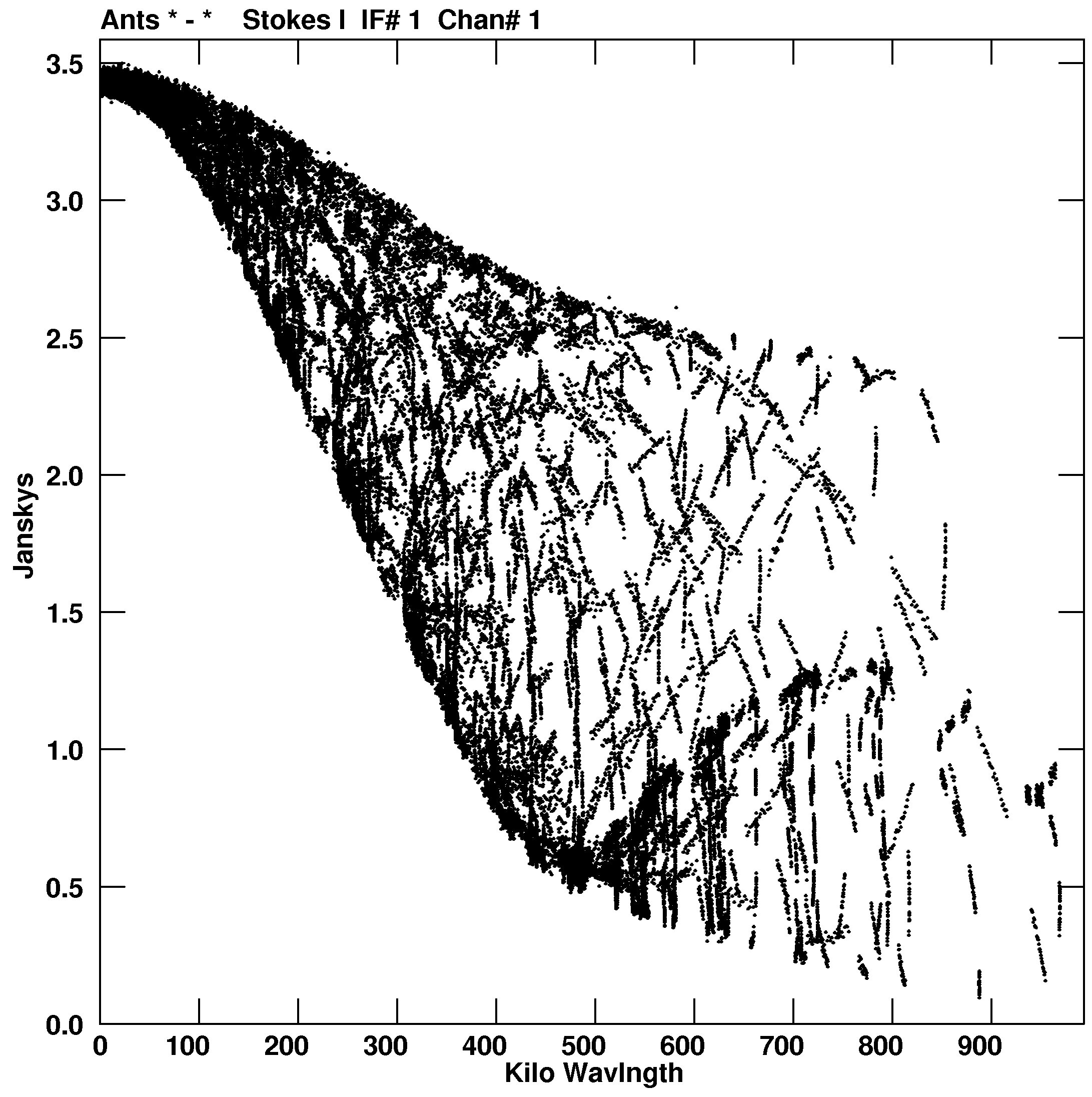
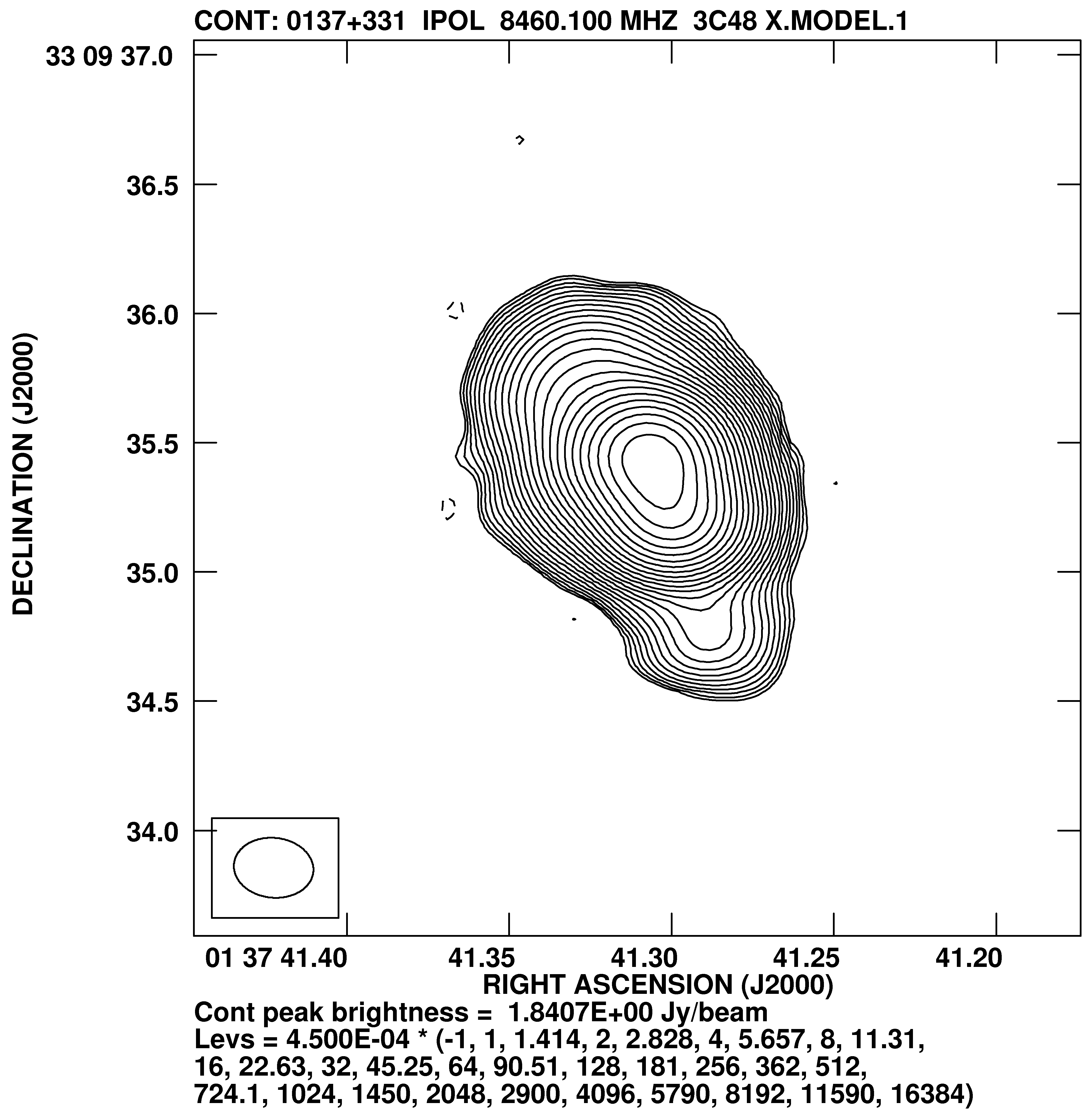
Unfortunately, since all the primary flux calibrators are resolved by the VLA in most configurations and at most
frequencies, they cannot be used directly to determine the amplitude calibration of the antennas without a detailed
model of the source structure, see Figure 4.1 as an example. Beginning in April 2004, model images for the
calibrators at some frequencies are included with . Models of 3C286, 3C48, 3C138, and 3C147 are available for
all 6 traditional bands of the VLA except 90 cm and even for S band of the EVLA. Type CALDIR C R to see a
list of the currently available calibrator models. Sources which are small enough to be substantially
unresolved by the VLA have variable flux densities which must be determined in each observing
session. A common method used to determine the flux densities of the secondary calibrators from the
primary calibrator(s) is to compare the amplitudes of the gain solutions from the procedure described
below.
Use SETJY to enter/calculate the flux density of each primary flux density calibrator. The ultimate reference for the VLA is 3C295, but 3C286 (1328+307), which is slightly resolved in most configurations at most frequencies, is the most useful primary calibrator. CALIB has an option that will allow you to make use of Clean component models for calibrator sources. You are strongly encouraged to use the existing models. If you follow past practice at the VLA, you may have to restrict the uv range over which you compute antenna gain solutions for 3C286, and may therefore insert a “phony” flux density appropriate only for that uv range at this point. In both cases, the following step should be done. CALIB will scale the total flux of the model to match the total flux of the source recorded by SETJY in the source table. This corrects for the model being taken at a somewhat different frequency than your observations and for the model containing most, but not all, of the total flux. An example of the inputs for SETJY, where you let it calculate the flux, would be:
> INP C R | to review inputs. |
> GO C R | when inputs okay. |
Or you can set the flux manually as shown below:
> SOURCES ’3C286’ , ’ ’ C R | if you used 3C286 as the source name. |
> ZEROSP 7.41 , 0 C R | I flux 7.41 Jy, Q, U, V fluxes 0. |
> INP C R | to review inputs. |
> GO C R | when inputs okay. |
> ZEROSP 7.46, 0 C R | I flux 7.46 Jy at the 2nd IF, Q, U, V fluxes 0. |
> GO C R |
|
Note that, although SOURCES can accept a source list, ZEROSP has room for only one set of I, Q, U, V flux densities. To set the flux densities for several different sources or IFs, you must therefore rerun SETJY for each source and each IF, changing the SOURCES, BIF, EIF, and ZEROSP inputs each time. Alternatively, set ZEROSP to the flux at 1 GHz and enter SPECINDX and SPECURVE adverbs to describe the dependence with frequency.
CALIB will use the V polarization flux in the source table if one has been entered. The RR polarization will be calibrated to I+V and the LL to I-V. While this has little practical use with circular polarizations because V is almost always negligible, it can be used for linearly polarized data from the WSRT. That telescope has equatorially mounted dishes, so the VV polarization is I-Q and the HH is I+Q independent of parallactic angle. For WSRT data, you should relabel the polarizations to RR/LL and enter I, 0, 0, -Q for ZEROSP, since Q is not negligible in standard calibrators.
In 31DEC22, more extensive calibration of linear polarization became available. CALIB will use the source table Q and U fluxes and the parallactic angles to compute proper gains for the V and H polarizations of point sources. A new procedure VHCALIB and task VHCAL have been written to apply full Clean-component polarization models to determine the parallel-hand gains of linear systems such a Meerkat.
If the LISTR scan listing shows calibration sources with a blank CALCODE, you should also use SETJY to correct this. Set OPTYPE = ’ ’, set the desired SOURCE name, and set CODETYPE to the desired CALCODE. Expert users sometimes prefer TABPUT for this function; run PRTAB to see what values must be set in PIXXY.
Bandpass calibration is for the modern VLA required rather than merely recommended. Having chosen those channels which may be reliably used to normalize the bandpass functions,
> DOCAL 1 C R | to apply the delay calibration — very important. |
> CALSOUR ’bandpass_cal’ C R | to select the strong bandpass calibrator. |
> SOLINT 0 C R | to find a bandpass solution for each scan on the BP calibrator. |
| to select the range(s) of channels which are reliable for averaging in each IF. Use the central 30% of the channels if your calibrators are all very strong or more like 90% if they are not. Remember these values — you will use them again. |
to normalize the results only after the solution is found using the channels selected by ICHANSEL. Use BPASSP(5)=-1 if your phases are not stable within each scan. Note that there are numerous options for BPASSPRM(10) including medians as well as means. |
> GO C R | to make a bandpass (BP) table. |
Do not use spectral smoothing at this point unless you want to use the same smoothing forever after. Apply the flag table. A model for the calibrator may be used; see §4.3.9.1.
Note: if your have a strong bandpass calibrator, observed frequently, you may use BPASS instead of CALIB to calibrate the gains. You must, if course, turn off the bandpass normaization entirely to use this option.
BPASS now contains the adverbs SPECINDX and SPECURVE through which the spectral index and its curvature (to higher order than is known for any source) may be entered. For the standard amplitude calibrators 3C286, 3C48, 3C147, and 3C138, these parameters are known and will be provided for you by BPASS. For other sources, you may provide these parameters, but BPASS will fit the fluxes in the SU table for a spectral index (including curvature optionally) if you do not. Note that, if no spectral index correction is applied, the spectral index of the calibration source will be frozen into the target source. Bandwidths on the EVLA are wide enough that this is a serious problem. If you do not know the spectral index of your calibration source, BPASS itself or the new task SOUSP may be used to determine the spectral indices from the SU table. Of course, that means that GETJY must already have been run. Since BPASS must usually be run before CALIB and hence GETJY, this suggests that one may have to iterate this whole process at least once. SOUSP now offers the option of correcting one or more SN tables after it adjusts the source fluxes for the spectral index it determined. This may reduce the need for further iterations.
Note that the bandpass parameters shown above assume that the phases are essentially constant through each scan of the bandpass calibrator. This may not be true, particularly at higher frequencies. In this case, you have two choices. One is to set BPASSPRM(5) to 0 which will determine the vector average of the channels selected by ICHANSEL at every integration and divide that into the data of that integration. This will remove all continuum phase fluctuations, but runs a risk of introducing a bias in the amplitudes since they do not have Gaussian statistics. BPASSPRM(5) = -1 now applies a phase-only correction on a record-by-record basis. A better procedure, which is rather more complicated, is as follows. Use SPLIT to separate the bandpass calibrator scans into a separate single-source file applying any flags and delay calibration and the like. Then run CALIB on this data set with a short SOLINT to determine and apply a phase-only self-calibration. On the uv data set written out by CALIB, run BPASS using the parameters described in the previous paragraph. Finally, use TACOP to copy the BP table back to the initial data set.
The spectral quality of the final images has been found to be determined in part by the quality of the bandpass solutions. In particular, for reasons which are not yet known, the bandpasses are not exactly antenna dependent especially in the edge channels. This “closure error” may be measured in individual and statistical ways by BPASS and reported to you. To check on this problem for your data set, set
> MINAMPER a C R | to count and, if BPASSPRM(2)> 1, to report amplitude closure failures > a per cent. Note that closure errors are accumulated as logarithms so that 0.5 and 2.0 are both errors of 100%. |
> BPASSPRM(2) 1 C R | to report statistics of amplitude and phase closure failures without reporting individual failures. |
> BPASSPRM(6) a C R | to report all channels in which the average amplitude closure error > a per cent. |
> BPASSPRM(7) p C R | to report all channels in which the average phase closure error > p degrees. |
> SOLTYPE ’R’ C R | to select robust solutions which discard data with serious closure problems. Try other types if there are solution failures. |
It is probably a good idea to set MINAMPER and MINPHSER fairly high (i.e., 20 and 12) to make a big deal only about major excursions, but to set BPASSPRM(6) and (7) fairly low (i.e., 0.5 and 0.5) to view the spectrum of closure errors (which will look a lot like the spectrum of noise on your final Clean images). There is even a task called BPERR which will summarize and plot the error reports generated by BPASS and written to text files by PRTMSG.
The bandpass solutions are calculated at each bandpass calibrator scan. As a consequence, they are likely to be unevenly spaced in time and may even have times (due to on-line or later editing) at which there are solutions for some IFs and polarizations but not all. When the latter happens, program source data will be lost unless the missing solutions are filled in. The task BPSMO may be used for this purpose or to create a new BP table at regular time intervals using one of a number of time-smoothing functions. Set APARM(4) = -1 for the “repair” mode or set APARM(4) to the desired BP interval.
After the bandpasses have been generated, you can examine them using tasks BPLOT and POSSM. You can obtain an average from all antennas with
> SOURCES ’cal1’ , ’cal2’ , … C R | to specify the bandpass calibrators. |
> ANTENNAS 0 C R | to include all antennas. |
> TIMER 0 C R | to average over all times. |
> BPVER 1 C R | to select the BP table. |
> FREQID 1 C R | to set the FQ value to use. |
> APARM = -1, 0 C R | to do a scalar average and have the plot self-scaled and labeled in channels. |
> APARM(8) 2 C R | to plot BP table data. |
> NPLOTS 0 C R | to make one plot only, averaging all included data. |
> INP C R | to review the inputs — check closely. |
> GO C R | to run the program when inputs set correctly. |
To view each antenna individually, using the TV to save paper
> NPLOTS 1 C R | to plot one antenna per page/screen. |
> GO C R | to display the bandpasses, averaged over time, on the TV with one antenna per screen. |
POSSM shows each screen for 30 seconds before going ahead. You can cause it wait indefinitely by hitting button A, speed it up by hitting TV buttons B or C, or tell it to quit by hitting button D. If DOTV = -1, then POSSM makes multiple plot extension files, which can be sent to the printer (individually or collectively) by LWPLA. You might want to use a larger value of NPLOTS to reduce the number of pieces of paper.
BPLOT is used to create one or more plots (on the TV or in plot files) of the selected bandpass table. The plots will be a set of profiles separated on the vertical axis by an increment in time or antenna number (depending on the sort selected). More than one plot for more than one antenna or more than one time may be generated. Multiple IFs and polarizations will be plotted along the horizontal axis if they are present in the BP table and selected by the adverbs. Thus, BPLOT is useful for plotting the change in bandpass shape as a function either of time or of antenna.
Task BPEDT offers a TV-interactive graphical way to check your BP table. It displays the amplitude and phase of one antenna to be edited and up to 10 more antennas for comparison. The task is like EDITA except that the horizontal axis is spectral channel rather than time. You may walk through the entire bandpass table selecting the editable antenna and time in sequence. If some of the solutions show residual effects from RFI, then you may generate flags in a flag table to delete certain spectral channels for certain antennas and times. If you do this, of course, you should re-run BPASS applying the new flags. In 31DEC21, BPEDT offers the option of flagging the BP values instead and even interpolating over the flagged values. Task BPFLG may be used with large BP tables after you have determined appropriate clip levels. Task BPEPL may be used to make plots similar to those of BPEDT without the interactivity. It will be faster if you have a lot of times in the BP table. If you do have lots of times in your BP table, BPPLT is another way to view a portion of the table as a function of time.
The BP tables are applied to the data by setting the adverb DOBAND > 0 and selecting the relevant BP table with the adverb BPVER. There are three modes of bandpass application. The first (DOBAND 1) will average all bandpasses for each antenna within the time range requested, generating a global solution for each antenna. The second mode (DOBAND 2) will use the antenna bandpasses nearest in time to the data point being calibrated. The third mode (DOBAND 3) interpolates in time between the antenna bandpasses and generates the correction from the interpolated data. This mode has been found to be required for VLA data. If BPSMO was used to make a fairly finely sampled BP table, then DOBAND 2 may be used. Modes DOBAND 4 and DOBAND 5 are the same as modes 2 and 3, respectively, except that data weights are ignored.
It is often not possible to observe a strong bandpass calibrator many times during a run. In this case, one can run BPASS on the single scan on the strong calibrator and then remove the main bandpass shape with DOBAND 1 in task SPLAT. Corrections to this basic bandpass shape as a function of time may then be determined with adequate signal-to-noise using task CPASS. This task can be used to fit the residual bandpass with a small number of parameters (<< the number of spectral channels) at each calibrator scan. The results may then be applied with DOBAND 2. Check the output of CPASS carefully — it is capable of making bandpass shapes with large ripples that are not present in the data. CPASS also knows about the flux coefficients of all standard sources and can fit the spectral index of other sources from the flux values in the SU table.
It is now considered standard practice to use flux calibrator models and you are strongly encouraged to do so. As
mentioned above, all the primary flux calibrators are resolved at most frequencies and configurations.
Figure 4.1 shows the visibilities and image of the commonly used calibrator 3C48 at X-band, it is
obvious this source is far from being point like. Since April 2004, source models have been shipped
with as FITS files. Currently, models for 3C48, 3C286 and 3C138 are available for all bands
except 90 cm and 3C147 at all bands except, X, C and P. Rick Perley has many models on two different
web sites, one for 2014 and one for 2019 observations. These may be reached in 31DEC20 by setting
DATAIN appropriately. Additional models are in the works, so you should always check to see what is
available:
> CALDIR C R | to list the available models by source name and band code. |
You can load a model with the procedure VLACALIB (see below) or you can load the model in manually using CALRD:
> OBJECT ’3C286’ C R | to load a model of 3C286. |
> VLOBS ’K’ C R | to select the available model at K band. |
> OUTDISK n C R | to write the model image and Clean components to disk n. |
> GO C R | to run the task and load the model. |
Set DATAIN = ’2019’ to select models from Perley’s 2019 website. Soon the task MOD3D will enable muti-facet models at P and 4 band to be distibuted with a “3D” model attached to a single facet.
The primary calibration task in is CALIB. Most of the complexity of CALIB can be hidden using the procedure
VLACALIB. Before attempting to use this procedure, you must first load it by typing:
Type HELP VLAPROCS for a full list of the procedures available in VLAPROCS.
The procedure VLACALIB automatically downloads and uses calibrator models, if one is available and the inputs are set correctly. After you have loaded VLACALIB you may invoke the calibrator model usage by setting:
> CALSOUR = ’Cala’ C R | to name one primary flux calibrator to invoke automatic calibrator model usage. |
> UVRANGE 0 C R | set to zero to invoke automatic calibrator model usage. |
> ANTENNAS 0 C R | set to zero to invoke automatic calibrator model usage. |
> REFANT n C R | reference antenna number — use a reliable antenna located near the center of the array. |
> MINAMPER 10 C R | display warning if baseline disagrees in amplitude by more than 10% from the model. |
> MINPHSER 10 C R | display warning if baseline disagrees by more than 10∘ of phase from the model. |
> FREQID 1 C R | use FQ number 1. |
> VLACALIB C R | to make the solution and print results. |
This procedure will load the calibrator model (using CALRD) and use it when it runs CALIB, then print any messages from CALIB about closure errors on the line printer, and finally run LISTR to print the amplitudes and phases of the derived solutions. Plots of these values may be obtained using task SNPLT.
Then you may select the model image with GET2N for use directly in CALIB. Example inputs for CALIB are:
> CALSOUR = ’Cala’ , ’ ’ C R | flux calibrator for which you have a model. |
> UVRANGE 0 C R | no uv limits needed. |
> ANTENNAS 0 C R | antenna selection not needed. |
> REFANT n C R | reference antenna number — use a reliable antenna located near the center of the array. |
> WEIGHTIT 1 C R | to select 1∕σ weights which may be more stable. |
> NCOMP 0 C R | to use all components. |
> SOLMODE ’A&P’ C R | to do amplitude and phase solutions. |
> APARM(6) 2 C R | to print closure failures. |
> MINAMPER 10 C R | to display warning if baseline disagrees in amplitude by more than 10% from the model. |
> MINPHSER 10 C R | to display warning if baseline disagrees by more than 10∘ of phase from the model. |
> CPARM(5) 1 C R | to vector average amplitudes over spetral channels and then scalar average them over time before determining solution. |
> FREQID 1 C R | to use FQ number 1. |
> GO C R | to make the solution. |
CALIB will use the clean components table attached to the model to find antenna gain solutions. It will sum the clean components within a certain radius of the center of the map (so that confusing sources that are part of the model do not influence the gain) and scale them to the flux in the SU table. Therefore, you must still run SETJY before running CALIB.
After running CALIB check the solutions for all antennas with SNPLT or LISTR (OPTYPE=’GAIN’). If you have multiple primary or secondary calibrators you will have to run CALIB separately for each, using models where they are available and restricting the UVRANGE and ANTENNAS where they are not. You can either write into the same SN table by setting SNVER to a table number or to different SN tables by setting SNVER = 0. Then you you can proceed as normal flagging and editing your data and proceed to final calibration as described in §4.3.10.
Normally, the primary flux calibration sources are located too far from the target sources to be used to track time variations in phase and amplitude. Therefore, secondary calibration sources whose fluxes and spectral indices are not known in advance.
Once you have read in procedure VLACALIB (see §4.3.9.1), you may use it to invoke CALIB. You will have to do this once for each calibrator, unless you can use the same UVRANGE for more than one of them. Thus,
> CALSOUR = ’Cala’ , ’Calx’ C R | to name two calibrators using the same UVRANGE and other adverb values. |
> UVRANGE uvmin uvmax C R | uv limits, if any, in kiloλ. |
> ANTENNAS list of antennas C R | antennas to use for the solutions, see discussion above. |
> REFANT n C R | reference antenna number — use a reliable antenna located near the center of the array. |
> MINAMPER 10 C R | display warning if baseline disagrees in amplitude by more than 10% from the model. |
> MINPHSER 10 C R | display warning if baseline disagrees by more than 10∘ of phase from the model. |
> FREQID 1 C R | use FQ number 1. |
> VLACALIB C R | to make the solution and print results. |
This procedure will first run CALIB, then print any messages from CALIB about closure errors on the line printer, and finally run LISTR to print the amplitudes and phases of the derived solutions. Plots of these values may be obtained using task SNPLT.
If the secondary calibrators require different values of UVRANGE, then CALIB must be run until it has run for all calibration sources. Attached to your input data set is a solution SN table. Each run of CALIB writes in this table (if SNVER = 1), for the times of the included calibration scans, the solutions for all IFs using the flux densities you set for your calibrators with SETJY or GETJY. (CALIB assumes a flux density of 1 Jy if no flux density is given in the SU table.) If a solution fails, however, the whole SN table can be compromised, forcing you to start over. It is possible to write multiple SN tables with SNVER = 0. Later programs such as GETJY and CLCAL will merge all SN tables which they find (if told to do so). Tables with failed solutions must be deleted.
Task GETJY can be used to determine the flux density of the secondary flux calibrators from the primary flux calibrator based on the flux densities set in the SU table and the antenna gain solutions in the SN tables. The SU and SN tables will be updated by GETJY to reflect the calculated values of the secondary calibrators’ flux densities. This procedure should also work if (incorrect) values of the secondary calibrators’ flux densities were present in the SU table when CALIB was run. Bad or redundant SN tables should be deleted using EXTDEST before running GETJY, or avoided by selecting tables one at a time with adverb SNVER.
To use GETJY:
> SOURCES ’cal1’ , ’cal2’ , ’cal3’ … C R | to select secondary flux calibrators. |
> CALSOU ’3C286’ , ’ ’ C R | to specify primary flux calibrator(s). |
> CALCODE ’ ’ C R | to use all calibrator codes. |
> FREQID 1 C R | to use FQ number 1. |
> ANTENNAS 0 C R | to include solutions for all antennas. |
> TIMERANG 0 C R | to include all times. |
> SNVER 0 C R | to use all SN tables. |
> INP C R | to review inputs. |
> GO C R | to run the task when the inputs are okay. |
GETJY will give a list of the derived flux densities and estimates of their uncertainties. These are now found by “robust” methods and additional information about numbers of aberrant solutions are given. If any of the uncertainties are large, then reexamine the SN tables as described above and re-run CALIB and/or GETJY as necessary. Multiple executions of GETJY will not cause problems as previous solutions for the unknown flux densities are simply overwritten. You may wish to run the task SOUSP to determine the spectral indices of your calibrators from their fluxes in the SU table. You can even replace the values in the SU table with the curve fit by SOUSP and correct the gains in one or more SN tables with the newly determined fluxes. These spectral index parameters may be useful in running BPASS and PCAL. However, BPASS knows the flux coefficients for all standard calibration sources and can fit the spectral index of other calibration sources from the SU table.
The task EDITA uses the graphics planes on the TV display to plot data from tables and to offer options for
editing (deleting, flagging) the associated uv data. Only the TY (VLB and historic VLA system temperature), SY
(modern VLA SysPower table), SN (solution), and CL (calibration) tables may be used. We recommend using EDITA
with the SN table updated by GETJY as a quick and easy way to examine the quality of the solutions. If a
small amount is disturbed, use EDITA to flag the relevant data. If the solutions for most antennas are
disturbed, make a note of the time and source and use other flagging tools to find and flag the cause of the
disturbance. If you flag more than a little, you should delete the SN table(s) and re-run VLACALIB and GETJY.
Try:
> INEXT ’SN’ C R | to use the solution table. |
> INVERS 0 C R | to use the highest numbered table, usually 1. |
> TIMER 0 C R | to select all times. |
to specify all IFs; you can then toggle between them interactively and even display all at once. |
> ANTENNAS 0 C R | to display data for all antennas. |
> FLAGVER 1 C R | to use flag (FG) table 1 on input. |
> OUTFGVER 0 C R | to create a new flag table with the flags from FG table 1 plus the new flags. |
> SOLINT 0 C R | to avoid averaging any samples. |
> DOHIST FALSE C R | to omit recording the flagging in the history file. |
to allow plots with all polarizations and/or IFs simultaneously, using color to differentiate the polarizations and IFs. The 2 speeds up the display. |
> INP C R | to review the inputs. |
> GO C R | to run the program when inputs set correctly. |
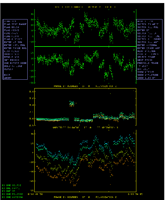
If you make multiple runs of EDITA, it is important to make sure that the flagging table entries are all in one version of the FG table. The easiest way to ensure this is to should set FLAGVER and OUTFGVER to 0 and keep it that way for all runs of EDITA. This may create an excessive number of flag tables, but unwanted ones may be deleted with EXTDEST. If you make a mistake two flag tables may be merged with the task TAPPE. A sample display from EDITA is shown on the next page.
The following discussion assumes that you have read §2.3.2 and are familiar with using the TV display. An
item in a menu such as that shown in the figure is selected by moving the TV cursor to the item (holding
down or pressing the left mouse button). At this point, the menu item will change color. To obtain
information about the item, press TV “button D” (usually the D key and also the F6 key on your
keyboard). To tell the program to execute the menu item, press any of TV buttons A, B, or C. Status
lines around the display indicate what is plotted and which data will be flagged by the next flagging
command. In the figure below, only the displayed antenna (2), and time range will be flagged. You must
display at least a few lines of the message window and your main AIPS window since the former
will be used for instructions and reports and the latter will be needed for data entry (e.g., antenna
selection).
The first thing to do with EDITA is to look at all of the polarizations, IFs, and antennæ, in order to make notes about disturbances in the solutions. Use SWITCH POLARIZATION to switch between polarizations and ENTER IF to select the IF to edit. Alternatively, NEXT POL/IF will cycle through all polarizations and IFs. If CROWDED was set to 1 or 2, SWITCH POLARIZATION will cycle through displaying both polarizations as well as each separately, and ENTER IF will accept 0 as indicating all. These options appear only if there is more than one polarization and/or more than one IF in the loaded data. Use ENTER ANTENNA to select the antenna to be flagged and ENTER OTHER ANT to select secondary antennæ to be displayed around the editing area. If the secondary antennæ have no obvious problems, then they do not have to be selected for editing. EDITA will plot all of the times in the available area, potentially making a very crowded display. You may select interactively a smaller time range or “frame” in order to see the samples more clearly. It is necessary to select each frame in order to edit the data in that frame so it helps to make the TV screen as big as possible with the F2 button or your window manager. Note that the vertical scales used by EDITA are linear, but that the horizontal scale is irregular and potentially discontinuous. Integer hours are indicated by tick marks and the time range of the frame is indicated. Use FLAG TIME or FLAG TIME RANGE to delete data following instructions which will appear on the message window. While you are editing, the source name, sample time and sample value currently selected will be displayed in the upper left corner of the TV screen.
Having noted all obviously bad points, you may now selectively flag visibility data. Select SWITCH ALL IF, SWITCH ALL TIME, SWITCH ALL ANT, SWITCH ALL POL, and SWITCH ALL SOURC so that the next flag command(s) apply to the portion of the data that should be flagged. The current setting of these toggles is displayed at the lower left corner. The various FLAG options allow you to flag single times, time ranges, all samples above or below a selected level, and single points either carefully or quickly. Finally, apply your flagging to your uv data set by selecting EXIT or throw it all away by selecting ABORT..
Note that it may also be profitable to run EDITA using the SY table. Unlike complex gains which reflect the values of all antennas, the SY values are strictly dependent only on the specific antenna. They are however affected by RFI in ways that may not affect the visibilities, so flagging uv data based on the SY values should be done with caution. EDITA, when run on SY or TY tables, has the option to display the difference of the current parameter with a running mean of that parameter. Such displays are a powerful editing tool.
At this point you should have gain and phase solutions for the times of all calibration scans, including the correct flux densities for the secondary calibrators. The next step is to interpolate the solutions derived from the calibrators into the CL table for all the sources. CLCAL may be run multiple times if subsets of the sources are to be calibrated by corresponding subsets of the calibrators, unless you limit it to one or more tables with SNVER and INVERS, CLCAL assumes that all SN tables contain only valid solutions and concatenates all of the SN tables with the highest numbered one. Therefore, any bad SN tables should be removed before using CLCAL. For polarization calibration, it is essential that you calibrate the primary flux calibrator (3C48 or 3C286) also so that you can solve for the left minus right phase offsets and apply PCAL.
CLCAL has caused considerable confusion and user error because it implements two somewhat contrary views of its
process. The older view, represented by previous versions of this  ook
ook ook, had the user gradually building a final
CL table from multiple runs of CLCAL, each with a selected set of calibration sources, target sources, antennas, time
ranges, and so forth. In this scheme, the user had to take great care that the final CL table actually contained
information for all antennas, sources, and times for which it would be needed. It was easy to get this wrong! The
second and now prevailing view is that every execution of CLCAL should write a new CL table containing all sources,
antennas, and times, but with a selected subset modified by the current execution. This leads to there being a
potentially large number of CL tables, but no data will be flagged due to the absence of data in the CL table.
The user will still have to be careful to insure that all CL records have received the needed calibration
information.
ook, had the user gradually building a final
CL table from multiple runs of CLCAL, each with a selected set of calibration sources, target sources, antennas, time
ranges, and so forth. In this scheme, the user had to take great care that the final CL table actually contained
information for all antennas, sources, and times for which it would be needed. It was easy to get this wrong! The
second and now prevailing view is that every execution of CLCAL should write a new CL table containing all sources,
antennas, and times, but with a selected subset modified by the current execution. This leads to there being a
potentially large number of CL tables, but no data will be flagged due to the absence of data in the CL table.
The user will still have to be careful to insure that all CL records have received the needed calibration
information.
To use CLCAL:
> SOURCES ’sou1’ , ’sou2’ , ’sou3’ , … C R | sources to calibrate, ’ ’ means all. |
> FREQID n C R | use FQ number n. |
> OPCODE ’CALP’ C R | to combine SN tables into a CL table, passing any records not altered this time. |
> GAINVER 0 C R | to select the latest CL table as input. |
> GAINUSE 0 C R | to select a new output CL table. |
> INTERP ’2PT’ C R | to use linear interpolation of the possibly smoothed calibrations.. |
> SAMPTYPE ’ ’ C R | to do no time-smoothing before the interpolation. |
> DOBLANK 1 C R | to replace failed solutions with smoothed ones but to use all previously good solutions without smoothing. |
> INP C R | to check inputs. |
Calibrator sources may also be selected with the QUAL and CALCODE adverbs; QUAL also applies to the sources to be
calibrated. Note that REFANT appears in the inputs because references all phases to those of the reference
antenna. If none is given, it defaults to the one used in the most solutions.
The smoothing and interpolation functions in CLCAL have been separated into two adverbs and the smoothing parameters are now conveyed with BPARM and ICUT. In smoothing, the DOBLANK adverb is particularly important; it controls whether good solutions are replaced with smoothed ones and whether previously failed solutions are replaced with smoothed ones. One can select either or both.
Note that CLCAL uses both the GAINUSE and GAINVER adverbs. This is to specify the input and output CL table
versions, which should be different. If you are building a single CL table piece by piece, then these
must be set carefully and normally held fixed. In the more modern view, they are set to zero and the
task takes the latest CL table as input and makes a new one. CL table version 1 is intended to be a
“virgin” table, free of all injury from any calibration you do using the package. It may not
always be devoid of information, as “on-line” corrections may be made and recorded here by some
telescope systems, e.g., the VLBA. The VLA, through tasks FILLM, BDF2AIPS, or INDXR, can now put
opacity and antenna gain information in this file. CLCAL and most other tasks are forbidden to
over-write version 1 of the CL table. This protects it from modification, and keeps it around so that you
may reset your calibration to the raw state by using EXTDEST to destroy all CL table extensions with
versions higher than 1. Be careful doing this, since you rarely want to delete CL version 1. Should
you destroy CL table version 1 accidentally, you may generate a new CL table version 1 with the task
INDXR. This new CL table may contain the calibration generated from the weather and antenna gain
files.
If you have any reason to suspect that the calibration has gone wrong — or if you are calibrating data for the first time — you should examine the contents of the output CL table. The task EVASN may help you determine the degree of phase and amplitude coherence in your calibration table. A lack of coherence suggests that the calibration is rather uncertain. Task SNPLT will provide you with a graphical display:
> INEXT ’CL’ C R | to examine the latest calibration table. |
> OPTYPE ’AMP’ C R | to examine amplitudes. |
to display all selected IFs in each plot using colors from red to blue. |
> INP C R | to check the inputs. |
> GO C R | to examine your CL table. |
Note that SNPLT may be used to examine SN, SY, and TY tables as well. OPCODE controls whether 1 IF or all IFs and 1 polarization or all polarizations are displayed. Task SNBPL will plot the calibration values on a baseline basis which can help to isolate the source of incoherence. SNFLG can be used to flag incoherent baselines rather than deleting whole antennas.
To test that the calibrators are actually properly calibrated by the new CL table, use UVPLT Try
> SOURCES ’cala’ ’ C R | to select calibrator sources one at a time. |
> BPARM 11 , 2 C R | to examine phase. |
> BPARM 11 , 1 C R | to examine amplitude. |
> DOTV 1 C R | to use the TV display. |
> GO C R |
|
You may need to limit which IFs are displayed or color the IFs with DO3COL 1. The phases should be near zero and the amplitudes should be nearly constant with baseline length. A decrease in the amplitude at the longest spacings indicates that the calibrator is not strictly a point source.
ANBPL converts baseline-based data before or after calibration into antenna-based quantities. In particular, the calibrated weights are very sensitive to problems with amplitude calibration.
> IND m ; GETN n C R | to specify the multi-source data set. |
> FREQID 1 C R | to select FQ value to image. |
> DOCALIB 1 C R | to apply calibration. |
> GAINUSE 0 C R | to use highest numbered CL table. |
> FLAGVER 1 C R | to edit data. |
> BPARM 2, 17 C R | to plot weight versus time. |
> DOCRT 0 C R | to suppress printed versions of the antenna-based values. |
> INP C R | to review the inputs. |
If the previous steps indicate serious problems and/or you are seriously confused about what you have done and you want to start the calibration again, you can use the procedure VLARESET from the RUN file VLAPROCS to reset the SN and CL tables.
> VLARESET C R | to reset SN and CL tables. |
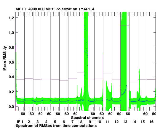
A very promising relatively new tool flags RFI on the assumption that it is either quite variable in time or in frequency. This task, called RFLAG, computes the rms over short time intervals in each spectral channel and IF individually and flags the interval whenever the rms exceeds a user-controlled threshold. Optionally, it will also use a sliding median window of user-specified width over the spectral channels to the real and imaginary parts of the visibility separately. Any channel deviating from the median in either part by more than a user-specified amount will also be flagged. If DOPLOT> 0, RFLAG will make plots of normal and cumulative histograms and of the mean and rms of the time and spectral computations as a function of channel. It will also make a flag table only if requested (DOFLAG> 0). These plots will suggest threshold parameters and allow you to choose values to use. A flag table is made for any value of DOFLAG if no plots are requested (DOPLOT≤ 0).
In detail, RFLAG is run using
> SOURCES ’source_1’, ’source_2’, … C R | to select sources of similar flux level. |
> STOKES ’FULL’ C R | to examine all polarizations. |
> FPARM 3 , x , -1, -1 C R | to examine spectral rms over 3 time intervals each a bit longer than x seconds. The -1’s cause the program to use other adverbs for the cutoffs and to do a spectral solution as well as the time one. |
to set the cutoff values as 4 times the median rms plus deviation found in the spectral plots as a function of IF. The default is 5. |
to flag all samples above x Jy and flag all of any channel with more than 0 ≤ y ≤ 1 of the time samples flagged. |
> FUNCTYPE ’LG’ C R | to plot the histograms on a log scale. |
> NBOXES 1000 C R | to use 1000 boxes in the histograms. |
> GO | to run the program. |
This will produce plots and set cutoff levels in adverbs NOISE and SCUTOFF. An example of the spectral plot is shown in Figure 4.3. Another run, with DOPLOT = 0 will apply these cutoffs and create a new flag table. Note that the flux cutoff levels may depend on the source flux, calling for different levels for strong calibrators, weak calibrators, and very weak target sources. Different cutoff levels for STOKES=’RRLL’ and STOKES = ’RLLR’ may also be needed. A strong, resolved target source may require different levels for different UVRANGEs. UVRANGE is now applied on a per spectral window basis so you no longer have to break up wide bandwidth data into multiple files when UVRANGE is required. RFLAG is a new task, so experiment a bit. Note that, if you set DOFLAG=1, the creation of a new flag table will happen after the plots in the same execution of RFLAG. If a channel is found bad at a time in any one polarization, all polarizations are flagged. If you have a significant spectral line signal in your data, use DCHANSEL to have the affected channels ignored throughout RFLAG or set FPARM(4) = 0 so that the spectral function is not performed.
There are a lot of adverbs to RFLAG. FPARM(5) allows you to speed up the spectral part of the flagging by testing more than just the central channel in the sliding median filter. FPARM(6) allows you to expand all flags to adjacent channels. FPARM(7), (8), (11), and (12) control the extending of flags to additional channels, baselines, or antennas if too large a fraction of channels, baselines, or baselines to an antenna are flagged in the basic time and spectral operations. Similar adverbs also occur in the new task REFLG whose job it is to compress the enormous flag tables generated generated by RFLAG. REFLG does not handle flags generated by CLIP, TVFLG, and SPFLG since they vary with polarization. REFLG can extend a flag to all times if too large a fraction of time is flagged for a given channel, baseline, etc. REFLG may not correctly compress all flags, but its other options are useful. The application of 10 million flag entries to a data set repetitively is rather expensive. Copying the data, applying the flags once and for all, is the best solution. RFLAG may now do this; set DOOUTPUT to true in 31DEC22 and later, along with output name adverbs OUTNAME, et al. UVCOP has been the traditional method to do this. However, TYAPL which needs to be run next and must make a new copy of the data has been given the option of applying a large flag table to avoid having to copy the data set twice. Task FGCNT lets you see how much of your data is flagged by any particular flag table. Task FGPRT will plot a matrix by baseline of the number of flags applying in a user specified range of time, spectral channel and IF, source, etc.
Having done a more careful job with your editing, it is now time to discard with EXTDEST the bandpass (BP) tables and all CL tables after the one written by VLANT. Discard all SN tables, but keep the highest numbered flag (FG) table.
Be very careful with the flag tables to save the last one - use IMHEADER to show you how many there are.
Because of its wide dynamic range, the EVLA does not normalize its output visibilities. To calibrate gains it records
the total power when the switched noise tube is on and when it is off. These data, taken in synchronism with the
visibilities, are recorded in the SysPower table of the ASDM. The OBIT program BDFIn, available to users in
the verb BDF2AIPS, reads this table and creates an SY table. The columns of this table contain POWER DIF
(Gain × (Pon - Poff), POWER SUM (Gain × (Pon + Poff)), and POST GAIN (Gain) columns for right and left
polarizations with values for each IF.
This table is accessible to users with a number of tasks. Begin with task PRTSY to view the table statistically
over time on a per IF, per antenna basis or to view scan or source median averages of one or more of the SY table
parameters. A more detailed look is available from SYPRT. Then to examine its contents graphically in various
ways, use SNPLT with OPTYPEs ’PDIF’, ’PSUM’, ’PGN’, ’PON’, ’POFF’, ’PSYS’, ’PDGN’, or ’PSGN’. You
could use OPTYPE = ’MULT’ to examine more than one of these at one time, comparing any oddities in
e.g., Psum and Pdif. Note that PSYS is especially interesting since Tcal * Psum∕(2 * Pdif) = Tsys, the
system temperature. It should reflect changes in elevation and strength of the observed source, but
should be immune to adjustments to the gain of the telescope. It determines data weights in TYAPL
while  divides into the visibilities. You may use EDITA (§4.3.11) to edit your uv data on the
basis of the contents of the SY table. Editing may be based on Psum, Pdif, Pgain, Tsys, and on the
differences between these parameters and a running median of these parameters. One may also edit the SY
table itself with SNEDT; the same parameters are available. LISTR can even display the SY table Psum,
Pdif, system temperatures, and gain factors with OPTYPE ’GAIN’ and DPARM(1) set to 17, 18, 15, or 16,
respectively.
divides into the visibilities. You may use EDITA (§4.3.11) to edit your uv data on the
basis of the contents of the SY table. Editing may be based on Psum, Pdif, Pgain, Tsys, and on the
differences between these parameters and a running median of these parameters. One may also edit the SY
table itself with SNEDT; the same parameters are available. LISTR can even display the SY table Psum,
Pdif, system temperatures, and gain factors with OPTYPE ’GAIN’ and DPARM(1) set to 17, 18, 15, or 16,
respectively.
In 31DEC25, a new experimental task SYHIS has become available. Unlike TYSMO, this task works on a per IF, per antenna, per polarization basis. It can plot histograms of the SY input table parameters. It can then clip the SY values, median-window filter the clipped data, plot histograms of the results, clip the median-window values, smooth the remaining values, and then replace the clipped samples (or all samples) with the smoothed values. These actionas are similar to those of TYSMO except that the task sets the clip levels separately for each antenna, IF, and polarization based on the values found in the histograms.
More importantly, the SY table can be used to do an initial calibration of the visibility data. Use the display programs to decide if your SY table is fine as is or needs editing. SNPLT may be the best way to examine The SY table. In 31DEC23, SNRMS may be used to determine the average values in the table and their rms. The following is somewhat controversial; there are users who believe that the SY table is never adequately reliable for all antennas because of RFI and other issues. Since the value of Tcal are not perfectly known, nor are the antenna efficiencies, the corrections made by TYAPL can never be perfect. Nonetheless, in many cases, they are a great help. CALIB will still be needed to finish the amplitude calibration.
The tasks TYSMO and TYAPL may be used with EVLA data having an SY table. TYSMO flags SY samples
on the basis of Pdif, Psum, Pgain, and Tsys and then smooths Psum, Pdif and Pgain to replace the
flagged samples and/or reduce the noise. You will want to do this to remove outlying bad points and
to reduce the jitter in these measurements. TYSMO even applies a flag table to the SY table before its
clipping and smoothing operations. Be sure to plot the results to make sure that the task did what
you wanted. It is both powerful and very helpful. Then use TYAPL to remove a previously applied SY
table (if any) and to apply the SY table you have prepared. The result should be data scaled nearly
correctly in Jy and weights in 1∕Jy2 in all IFs. The CUTOFF option allows you to use obviously good
values from the SY table while passing the data from antennas with poor SY values along unchanged.
If the SY values from some polarizations or IFs are bad due to RFI while others are good, you may
copy the good values to replace the bad values using task TYCOP. The wide-band, 3-bit mode of the
EVLA has serious non-linearities in the Pdif measurements which are not yet fully understood. For
such data, use OPTYPE=’PGN’ to apply only the post-detection gains to the data. This will remove
abrupt jumps due to changes in those gains (which will be more common with 3-bit data). Note that
TYSMO and TYAPL also require a table of the Tcal values which OBIT provides in an CD table.
Amplitude calibrations are not applied to EVLA data weights until they have been made meaningful by
TYAPL or REWAY. Set FLAGVER in TYAPL if you want to apply your flag table once and for all. TYAPL can
handle flag tables much larger than those that many other tasks can handle. Note that TYAPL must copy
the data set since it makes corrections to the antennas on very short intervals (not suitable to a CL
table).
If you have observations of the Sun, do not use TYAPL; use SYSOL instead. This task does the usual TYAPL operation
on non-Solar scans, but, for Solar scans, it must determine the average gain and weight factors on those antennas
having solar Tcals and then apply those averages to all antennas not equipped with Solar Tcals. Use a well-edited SY
table if possible. This Solar capability was made available in OBIT (version 567) and in mid-June 2017. The
revised format of the SY table includes a column to tell tasks whether to use normal or solar Tcals for that row of the
table.
You may skip this section unless you have cross-hand polarization data and wish to make use of them. Although
there have been major improvements in polarization routines, they still do not correct parallel hand
visibilities for polarization leakage. Thus you need to calibrate polarization only if you wish to make images of
target source Q and U Stokes parameters. Note that we discuss here the calibration of both linear and circular
polarization with tasks TECOR, RLDLY, and PCAL. At the phase difference stage, however, the process for linear feeds
is different than for circular feeds.
The calibration of wide-band visibility data sensitive to polarization involves three distinct operations: (1) determining and correcting the offset in delay between the two parallel-hand polarizations, (2) determining and correcting the data for the effects of imperfect telescope feeds, and (3) removing any systematic phase offsets between the two systems of orthogonal polarization. These three components of polarization calibration will be considered separately.
Faraday rotation in the Earth’s ionosphere can add a phase difference between the two parallel-hand polarizations
which is both time and direction dependent. These are particularly important at lower frequencies (< 4GHz), but
may rarely affect higher frequency-data as well. One way to remove at least some of the ionospheric phase offsets is
by applying a global ionospheric model derived from GPS measurements. The task TECOR processes such
ionospheric models that are in standard format known as the IONEX format. These models are available
from the Crustal Dynamics Data Information System (CDDIS) archive. There is a procedure which is
part of VLAPROCS, called VLATECR that automatically downloads the needed IONEX files from CDDIS
and runs TECOR. It will examine the header and the NX table and figure out which dates need to be
downloaded, so the observation date in the header must be correct and an NX table must exist. See
EXPLAIN VLATECR for other requirements. The default TECRTYPE is jplg which seems to work well for the
VLA.
to acquire the procedures; this should be done only once since they will be remembered. |
> APARM 1,0 C R | to apply dispersive delay corrections which may be useful for wide bandwidths. The remaining APARM values appear to work well for the VLA when left at 0. |
> VLATECR C R | to run the procedure. |
TECOR applies its corrections to the highest numbered CL table and writes a new one. A significant bug fix was made in January 2023 and applied retroactively to the 31DEC21 and 31DEC22 releases. TECOR now writes a “TE” table which may be plotted with TEPLT to examine all details of this correction. The new task MFIMG may also be used to make an image of the TEC data or the model used for the Earth’s magnetic field in TECOR. All standard image displays may then be used to view the results.
Extensive studies have revealed that TECOR usually over-corrects VLA data. It removes the time-dependent IFRM but leaves behind an extra rotation measure that changes some with obsering date and very slightly with source. A package of software called ALBUS has been found to give somewhat better solutions for the IFRM. In 31DEC24 a task also named ALBUS was written to invoke this package to correct uv data including dispersive delay which is important to VLBI data. Unfortunately, the complications of this package require the Linux operating system and an outside program called apptainer. See EVLA Memo 235 for details.2
Frequently, the delay difference between right- and left-hand, or V and H, polarizations must be determined even if FRING was not required for the parallel-hand data. Use POSSM to plot the RL and LR (or VH and HV) spectra to see if there are significant slopes in phase. If so, use a calibration source with significant polarization, although the EVLA D terms are often large enough to provide a usable signal in the absence of a real polarized signal. Note that 3C286 is significantly polarized and is likely to be the best source to use for this purpose. Then
> REFANT nr C R | to select a reference antenna - only baselines to this antenna are used so select carefully. Alternatively, REFANT 0 will loop over all possible (not necessarily good) reference antennas, averaging the result. |
> DOIFS j C R | to set the adverb to the value of APARM(5) used in FRING (§4.3.6. The IFs are done independently (≤ 0), all together (= 1), in halves (= 2), or more generally in N groups (= N). A value of -1 causes RLDLY to use BPARM to define the IF groupings, as in FRING. |
| to specify the beginning day, hour, minute, and second and ending day, hour, minute, and second (wrt REFDATE) of the data to be included. Use an interval not unlike the one you used in FRING. |
> INP C R | to check the inputs. |
> GO C R | to produce a new SN table with a suitable left polarization delay. |
Note that RLDLY now always creates an SN table and may be run with multiple calibrator scans. If there is only one calibrator scan and APARM(2)≤ 0, it will also copy the CL table which was applied to the input data through GAINUSE to a new CL table applying the correction to the L polarization delay. For all other cases, you must apply the added L polarization delays with CLCAL.
To begin with, it is probably better to determine a continuum solution for source polarization and antenna D terms before doing the lower signal-to-noise spectral solutions. To find an average solution for each IF:
> CALSOUR ’pol_cal1’, ’pol_cal2’ C R | to select the polarization calibrator(s) by whatever form of their names appears in your LISTR output. These sources must have I polarization fluxes in the source table. |
| to select the range(s) of channels which are reliable for averaging in each IF. These probably should be the same values that you used in BPASS. |
> PRTLEV 1 C R | to see the answers and uncertainties on an antenna and IF basis. |
> CPARM 0,1 C R | to update the source table with the calibrator source Q and U found. |
> INP C R | to review the inputs. |
> GO C R | to find the antenna leakage terms and the source Q and U values on an IF-dependent basis. |
PCAL will write the antenna leakage terms in the antenna file and the source Q and U terms in the source table (if CPARM(2) > 0). DOMODEL may be set to true only if the model has Q = U = 0 since PCAL cannot solve for the right minus left phase difference. If SOLINT=0, PCAL will break up a single scan into multiple intervals, attempting to get a solution even without a wide range of parallactic angles.
Use TASAV to copy all your table files to a dummy uv data set, saving in particular the CL table with the results of the amplitude and phase calibration. This step is not essential, but it reduces the magnitude of the disaster if the the next step fails in some way. (Note - this may be a good idea at several stages of the calibration process!)
> CLRO C R | Use default output file file name. |
> INP C R | to review the (few) inputs. |
> GO C R | to run the program. |
The task TACOP may be used to recover any tables that get trashed during later steps. Note that the next step writes a new CL table, but changes the AN and SU tables in place.
Having prepared a continuum solution for Q and U, you must also correct it for the difference in phase between R and L (or V and H) polarizations which normally varies considerably between IFs. For circularly polarized feeds only, the task RLDIF will correct the antenna, source, and calibration tables for this difference using observations of a source with known ratio of Q to U. 3C286 is by far the best calibrator for this purpose.
> DOPOL 1 C R | to apply the polarization calibration. |
> SOURCES ’pol_cal1’, ’pol_cal2’ C R | to select the polarization calibrator(s) by whatever form of their names appears in your LISTR output. These sources must have known polarization angles. |
> SPECTRAL 0 C R | to do the correction in continuum mode. |
> DOAPPLY 1 C R | to apply the solutions to a CL table (making a new modified one) and to the AN and SU tables, updating them in place. |
> DOPRINT 0 C R | to omit all the possible printing. |
> INP C R | to review the inputs. |
> GO C R | to determine and apply the corrections. |
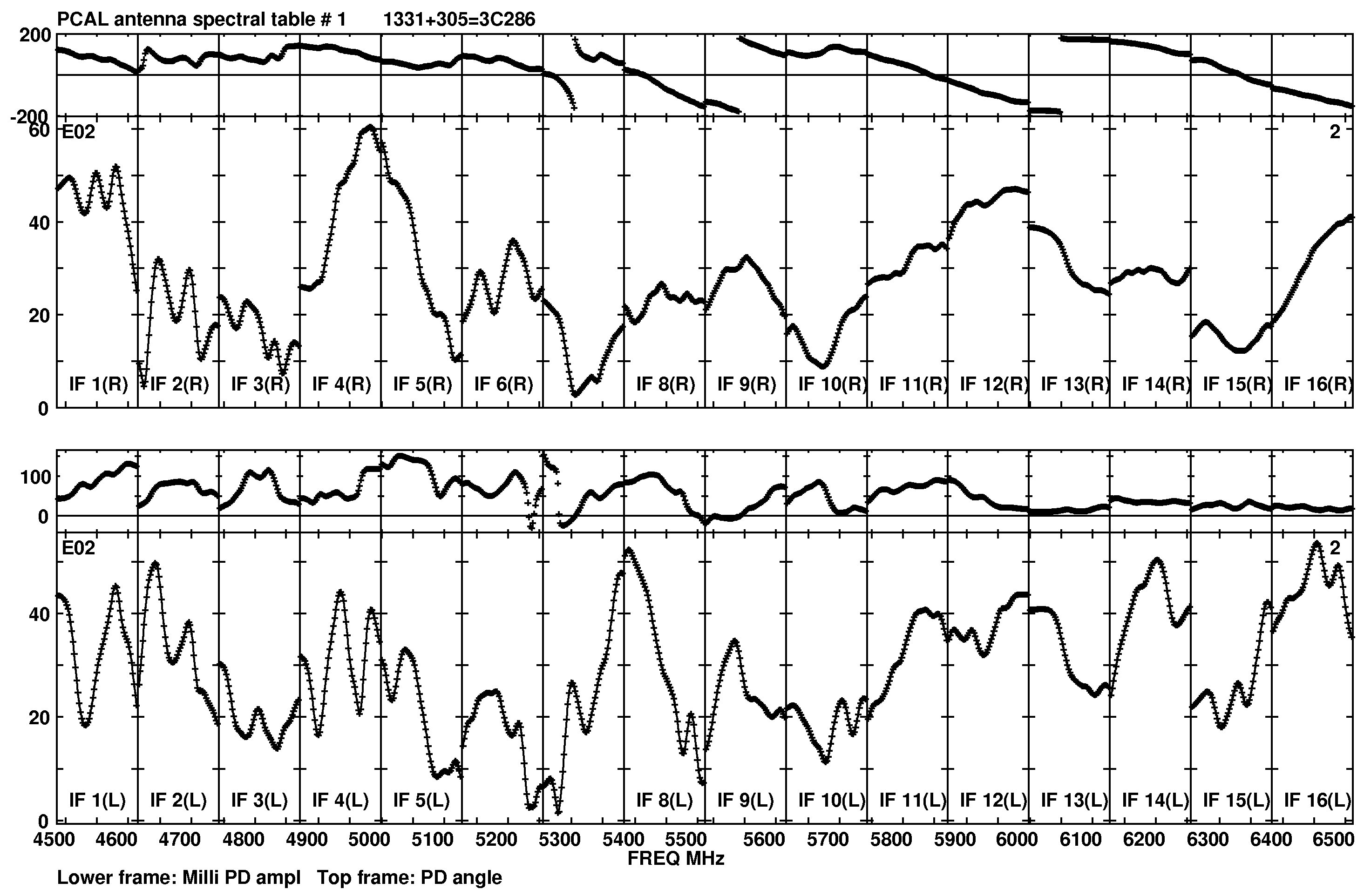
The EVLA polarizers appear to be very stable in time, but to have significant variation with frequency. See Figure 4.4. Serious polarimetry with the EVLA will require solving for the antenna polarization leakage as a function of frequency. To compute a spectral solution, assuming you already did the process in the preceding paragraph:
> SPECTRAL 1 C R | to do the channel-dependent mode. |
> DOMODEL 0 C R | to solve for Q and U as a function of frequency. Because PCAL does not solve for a right-left phase difference and that difference is a function of spectral channel, you must solve for a source polarization. |
> SPECPARM 0 C R | to determine the calibration source I, Q, and U spectral indices from fluxes in the source table. If you use PMODEL you must provide spectral indices for the model that apply in the frequency range of the data (curvature cannot be specified). |
> INTPARM p1,p2,p3 C R | to smooth the data after all calibration has been done while honoring ICHANSEL. |
> INP C R | to review the inputs, the task will take a while to run. |
> GO C R | to run the task writing a PD table of spectral leakages (“D terms”) and, if DOMODEL ≤ 0, a CP table of source Q and U spectra. |
If the combination of flagging, ICHANSEL, and INTPARM results in no solutions for some channels, the solutions from nearby channels will be interpolated or extrapolated so that all channels get solutions. If the calibration source is known to have no polarization, then you may set DOMODEL 1 and set PMODEL = flux , 0. Note that PCAL does not solve correctly for polarization when run on linearly-polarized data. You must use an unpolarized calibration source on such data sets. See below for a new way to get out of this problem.
After running PCAL in spectral mode, you may examine the resulting PD (polarization D terms) table with POSSM using APARM(8)=6 and BPLOT using INEXT = ’PD’. To compare two or more PD tables, use task PDPLT in 31DEC20. If a CP table (calibrator polarization) was written, you may also use POSSM with APARM(8) = 7 or 8 and BPLOT with INEXT = ’CP’ to examine the results.
You are almost, but not quite done. The combination of CALIB and BPASS has produced a good calibration for everything except the phase difference between right and left polarizations. This is now a function of spectral channel and needs to be corrected. The task RLDIF has been modified to determine a continuum or spectral right minus left phase difference and to modify the CL or BP table, respectively, to apply a phase change to the left polarization on an IF or channel, respectively, basis. Thus
> DOPOL 1 C R | to apply the polarization calibration, spectral if present. |
> INTPARM p1,p2,p3 C R | to smooth the data after all calibration has been done. |
to use solutions from channels c1 through c2 only, extrapolating solutions to channels outside this range. |
> SOURCES ’pol_cal1’, ’pol_cal2’ C R | to select the polarization calibrator(s) by whatever form of their names appears in your LISTR output. These sources must have known polarization angles. |
> POLANGLE p1,p2 C R | to provide the task with the source polarization angle(s) in degrees in source number order. The phase correction will be twice this value minus the observed RL phase. Do not provide values for 3C286, 3C147, 3C48, and 3C138. These are known to RLDIF including rotation measures and other spectral dependence. |
> ROTMEAS r1 C R | to provide in 31DEC23, the rotation measure in radians per meter squared for the first calibration source. |
> SPECTRAL 1 C R | to do the correction in spectral mode. |
> DOAPPLY 1 C R | to apply the solutions to a BP table (making a new modified one) and to the PD and CP tables. |
to write the phase corrections applied to a text file suitable for plotting by PLOTR. |
> INP C R | to review the inputs. |
> GO C R | to determine and apply the corrections. |
The right minus left phase difference may be a modest (we hope) function of time. To have RLDIF solve for this, set adverbs DOKEEP = 1 to invoke this option, SOLINT to an averaging time in minutes, and ICHANSEL as needed. The applied PP table will still be the global average solution, but individual time interval solutions will be written to the PP table and may be plotted with POSSM. An SN table is written so that the channel average right minus left phase may be applied as a function of time and IF to the CL table if desired.
Note that RLDIF applies to circularly polarized feeds only and requires you to know the linear polarization angle of at least one calibration source. The methods for calibrating linearly-polarized feeds, which are only at P- and 4-bands on the VLA, are still being developed. It appears that one requires one or more calibration sources known to have polarization in Stokes U and to have no emission in Stokes V (circularly-polarized emission). If you have such data, then the new task VHDIF performs the functions of RLDIF for linear feeds. 3C345 is such a calibration source, but at P-band its rotation measure makes the U polarization very weak at some frequencies while it is strong enough at others. Task PPAPP may be used to apply SPECTRAL > 0 tables to the BP tables of additional data sets.
In 31DEC24, a new task VH2RL may help in calibrating linear polarization in . It translates linear polarization
data into circular. In order to do this, there are a number of requirements. There must be all 4 correlations in the
data which must be calibrated by at least BPASS in its unnormalized mode (or use CALIB also), RLDLY, and VHDIF.
Use an unpolarized source for BPASS, CALIB, and RLDLY; there are many at P-band. After applying VH2RL, you
may then calibrate with additional, linearly-polarized sources and run PCAL and RLDIF in the normal
way.
Task SNP2D will help calibrate data sets which contain a strong, e.g., maser, line in one or a few channels with interesting but weaker signals in other channels and/or the continuum. After applying the best standard calibration described above, you can split out the maser channel(s) with UVCOP. Make images and self-calibrate following the processes described in Chapter 5 making an SN table containing the full calibration needed to apply to the maser. Then use task SNP2D to convert this into delays and phases to apply to the full, multi-IF data set. This will work so long as the residual phases found in the self-cal are small and is actually required to do the best calibration possible over very wide bandwidths.
For the historic VLA, FILLM was able to compute meaningful data weights which were then improved with the amplitude calibration. For the EVLA, however, the data weights begin as solely the integration time. For 8-bit data, TYAPL (§4.3.15) is able to convert these into meaningful weights. However, if TYAPL was used only with OPTYPE = ’PGN’, or not used at all, then it behooves you to rectify the situation. There is a task called REWAY which computes a robust rms over spectral channels within each IF and polarization. It can simply base the weights on these on a record-by-record, baseline-by-baseline basis. Alternatively, it can use a scrolling buffer in time so that the robust rms includes data for a user-specified number of records surrounding the current one. A third choice is to average the single-time rmses over a time range and then convert them to antenna-based rmses. In all three modes, the task can then smooth the rmses over time applying clipping based on user adverbs and the mean and variance found in the rmses. A flag table (extension file) may be written to the input data file removing those data found to have rmses that are either too high or too low. For these weights to be meaningful, the bandpass and spectral polarization calibration must be applied and it helps to omit any RFI or other real spectral-line signal channels from the rms computation. For the weights to be correctly calibrated, all amplitude calibration must also be applied. For these reasons, REWAY might well be used instead of SPLIT — when TYAPL was not used — running it one source at a time. Thus,
> SOURCES ’target1’ , ’ ’ C R | to do one target source. |
> APARM 11, 30, 12, 0, 10, 4 C R | to use a rolling buffer of 11 times separated by no more than 30 seconds and then smoothed further with a Gaussian 12 seconds in FWHM. Data are flagged if the rms is more than 4 times the variance away from the mean averaged over all baselines, IFs, and polarizations. Flagging on the variance of the rms from the mean on a baseline basis is essentially turned off by the 10. |
> GO C R | to write out a calibrated, weighted data set for the first target source. |
Then, when that finishes
It is not clear that this algorithm is optimal, but it certainly should be better than using all weights 1.0 throughout. It will be interesting to compare data weights found with TYAPL to those found with REWAY. The task now displays statistical information to assist the user in determining which weights are excessively high or low.
With the historic VLA, spectral-line observations were normally done with frequencies which changed with time in order to track a chosen source velocity at a specific spectral channel. The narrow bandwidths of the historic VLA kept this operation out of non-linear regimes. The EVLA, however, has very wide bandwidths, making the appropriate frequency changes different for each spectral window. For spectral imaging, however, this frequency shift must be done, at least for narrow bandwidths, long observing sessions, or combinations of multiple observing sessions. It is probably best to separate out the spectral window (IF) containing the desired spectral line signals and do the following on that window alone.
At present, the EVLA observing setup allows you to select the initial frequency of observation based on a desired LSRK velocity in the central channel. From there, however, the observations are conducted at a fixed frequency. Furthermore, the information about rest frequencies, source velocities, and even more fundamental parameters such as reference frame (LSRK or barycentric) and type of velocity (radio or optical) are lost. SETJY allows you to correct this. First use SETJY to set the desired rest frequencies (note that they are allowed to be a function of IF) and the VELTYP and VELDEF. Then use OPTYEP=’VCAL’ over all sources and IFs. This will compute the velocities at which you observed for the first time you observed each source and enter the values in the source table.
Having done this, the task CVEL may be used to shift the visibility data to correct for the rotation of the Earth about its axis as well as the motion of the Earth about the Solar System barycenter and the motion of the barycenter with respect to the Local kinetic Standard of Rest. CVEL works on multi-source as well as single-source data sets. It applies any flagging and bandpass calibration to the data before shifting the velocity (which it does by a carefully correct Fourier transform method). Note, the use of Fourier-transforms means that one must not use CVEL on data with channel separations comparable to the widths of some of the spectral features. Furthermore, narrow EVLA bands apparently have sharp cutoffs at the edges which cause any continuum signal to generate sine waves in amplitude after the FFT. Therefore, UVLSF must be run before CVEL. The velocity information used by CVEL must be correct. Use LISTR and SETJY to insure this before using SPLIT and CVEL. A special version of CVEL has been written to correct not only for the Earth’s motion but also for planetary motion to observe a line at rest with respect to a planet; see PCVEL.
IMAGR can be used to make images from multi-source data files. It is probably a good idea to make a couple of quick images to make sure that the calibration is okay. An example set of inputs to IMAGR for a continuum image is:
to select task and initialize all its parameters. This selects the usual convolution and weighting functions among other things. |
> IND m ; GETN n C R | to specify the multi-source data set. |
> SRCNAME ’sou1’ , ’ ’ C R | to choose one source to image. |
> FREQID 1 C R | to select FQ value to image. |
> NCHAV (m - n + 1) C R | to include all spectral channels plus IFs bif through eif in each image. Note that each channel and IF included in the “average” image is handled individually at its correct frequency. |
> GAINUSE 0 C R | to use highest numbered CL table. |
> FLAGVER 1 C R | to edit data. |
> DOBAND 3 C R | to correct bandpass with time smoothing. |
> BPVER 1 C R | to select BP table to apply. |
> OUTNAME ’sou1’ C R | to set the output file name to the source name. |
> OUTDISK 0 C R | to use any output disk with enough space. |
> IMSIZE 512 512 C R | to set the size in cells of image. |
> CELLSIZE 0.25 , 0.25 C R | to set the size of each image cell in arc-seconds. |
> UVWTFN ’ ’ C R | to use uniform weighting. |
> ZEROSP 0 C R | to introduce no zero-spacing flux. |
> NITER 0 C R | to do no Cleaning. |
> INP C R | to review the inputs. |
Note that some of the above values are set by DEFAULT but we wish to emphasize the parameters here. The CELLSIZE and IMSIZE depend on your data; use SETFC to make recommendations.
After you have edited your target sources with RFLAG and checked the calibration with IMAGR, your calibration is complete — at least until you do self-calibration. It is probably time to back up your data. You may wish to apply the final large flag table from RFLAG before backing up the data. Use UVCOP to apply especially large flag tables, but be sure to copy all of your data otherwise. Then
> IND m ; GETN n C R | to specify the multi-source data set. |
> DATAOUT ’logical:filename C R | to specify the output disk file name in the usual manner; see §3.10.3 |
> DOPLOT 1 C R | to include plot files. |
> INP C R | to review the inputs. |
> GO C R | to write a “uvfits” file on disk. |
Task FITAB writes a variant of this format in which the visibility data are also written in a FITS table
format. The FITAB form is preferred esthetically by some, but most other software packages cannot
read it properly. The FITS format used for plot files in 31DEC24 will not be useful to any sotware
other than . The FITS format used by is extensively documented in Memo
117.3
When you are happy with the and editing represented by the current set of calibration and flag tables, you can convert the multi-source file into single-source files, applying your calibration and editing tables. Remember that only one FREQID can be SPLIT at a time.
> SOURCES ’sou1’ , ’sou2’ , … C R | to select sources, ’ ’ means all. |
> TIMERANG 0 C R | to keep all times. |
> FREQID 1 C R | to set the one FQ value to use. |
> DOCALIB 1 C R | to apply calibration to the data and the weights. |
> GAINUSE 0 C R | to use the highest numbered CL table. |
to correct for feed polarization, but only if you solved for the polarization in §4.3.16. |
> DOBAND 3 C R | to correct bandpass with time smoothing. |
> BPVER 1 C R | to select BP table to apply. |
> STOKES ’ ’ C R | to write the input Stokes type. |
> DOUVCOMP FALSE C R | to write visibilities in uncompressed format. |
> APARM 0 C R | to avoid channel averaging and autocorrelation data. |
> INP C R | to review the inputs. |
> GO C R | to run the program when inputs set correctly. |
The files produced by this process should be completely calibrated and edited and ready to be imaged or further processed as described in later chapters. Note that one may wish to defer the DOPOL 1 part of this until after self-calibration of the parallel-hand visibilities. When finally applying the polarization calibration, the option of applying a rotation measure to the cross-hand data is offered. This will make the cross-hands not represent what was measured, but instead represent a value at frequency 0. Removing a known rotation measure, however, then allows averaging over frequency in Q and U for better signal-to-noise.