6.3 Plotting your data

The basic concept in ’ plotting is to use some task to create and write a device-independent plot file as a PL extension file to a cataloged image or visibility data set and then to use some device-dependent task to interpret that file for the desired output device. Plot files are not overwritten by subsequent plot tasks. Instead they make new plot files with higher “version” numbers. The device-dependent tasks include TVPL ( TV devices including XAS), TKPL (Tektronix graphics devices including ’ TEKSRV server), TXPL (line printers), and LWPLA (PostScript printer/plotters). Tasks called PRTPL, QMSPL, and CANPL support antique Versatec, QMS, and Canon printer/plotters. To plot on a PostScript printer/plotter:

LWPLA offers the option to save the file for later plotting or inclusion as encapsulated PostScript in other documents. It also has options to control scaling, output paper size, width and darkness of lines, and transformation of grey-scale intensities. It can write more than one plot file at a time and can append new plots to existing output files. Multi-plot files are not “encapsulated” but may be printed and viewed with tools such as gv or ghostview. Note that PostScript files are text files and  writes particularly simple PostScript so that it can be modified by the users. See HELP POSTSCRIPT for suggestions including information on deleting and adding labels and arrows and on converting the PostScript to other formats like jpg without loss of resolution.

LWPLA and all plot tasks offer some “coloring” options. These are illustrated in the color pages at the end of this chapter. The grey-scale plotting tasks, including GREYS, PCNTR, and KNTR, can now enhance the grey-scales with a transfer function and then pseudo-color them with a color table. See §6.4.3 for a short discussion of “output-function memory” tables which may be read into the above tasks or to LWPLA using the adverb OFMFILE. Lines plotted on top of grey scales (e.g., contours, polarization vectors, stars) may be “dark” when the grey scale intensity is high. LWPLA may be instructed to plot these as bright if adverb DODARK is false. All plot programs can draw lines of different types in both bright and dark forms. In LWPLA, if DOCOLOR is true, the array adverb PLCOLORS(i,j) controls the red, green, and blue colors (i = 1,2,3, resp.) of line types j = 1 – 10. The normal meanings of these types are:

1.  Bright labeling, tick marks, surrounding lines
2.  Bright lines, usually contours or model curves
3.  Bright lines, usually polarization vectors
4.  Bright lines, usually symbols such as stars, visibility samples
5.  Dark labeling text inside plot area
6.  Dark lines, usually contours
7.  Dark lines, usually polarization vectors
8.  Dark lines, usually symbols such as stars
9.  Bright labeling outside the main plot area, e.g. titles, tick values and types, documentation
10.  Background for the full plot

Some plot tasks have the ability to control the colors of their line drawing independent of these line types. These colors may be controlled only when making the plot file with the particular task. PCNTR and KNTR have acquired the ability to color each contour level under control of the adverb RGBLEVS. Using system RUN file SETRGBL, procedures CIRCLEVS, RAINLEVS, FLAMLEVS, and STEPLEVS are available to help you set the values of RGBLEVS. Examples are shown on the color pages at the end of this chapter. With LWPLA and these options one may prepare extremely effective displays — or hopelessly bad ones — for use in talks and, since the prices have become reasonable, even in journals. Note that most journals want color images in CMYK (cyan-magenta-yellow-black) rather than RGB; use DPARM(9) = 1 in LWPLA to get PostScript files with this color convention. Note that these two color representations usually require different “gamma” corrections; the adverb RGBGAMMA allows this control in LWPLA.

All  plot tasks now offer a “preview” option. If you set DOTV = TRUE when running any plot task, then the plot appears immediately on the  TV display and no plot file is generated. This option allows you to make sure that the parameters of the plot are reasonable and lets you avoid making files and wasting paper for quick-look plots. Additional options allow you to control which graphics channel is used for the line drawing (GRCHAN) and to select pixel scaling of the plot at your specified location on the TV screen (TVCORN). These two options allow you to view more than one plot at a time on the TV, usually for purposes of comparison. Each graphics channel on the TV has a different color and a complementary color is used when two or more channels are on at the same point. This allows for a fairly detailed and effective comparison of plots, all of which may be captured with task TVCPS (see below). Be aware that most tasks now interpret GRCHAN = 0 as an instruction to use graphics channels 1 through 4 for line types 1 through 4 and graphics channel 8 for dark vectors. The comparison function is only achieved by specifying GRCHAN; see HELP GRCHAN for more information. Tasks that produce multiple plot files pause for 30 seconds at the end of each plot when DOTV = TRUE. This allows you to stop the task (TV button D), hurry it along (TV buttons B or C), or make it pause indefinitely (TV button A) until another TV button is pressed.

You can review the parameters of the plot files associated with a given image or visibility data set by typing:

Plot files (and other “extension files”) are automatically deleted when an image is deleted by ZAP. However, large plot files should be deleted as soon as they are no longer needed:

Plot files are not amenable to the FITS format and so are not written by FITTP and FITAB. They may be copied from one catalog entry to another with TACOP.

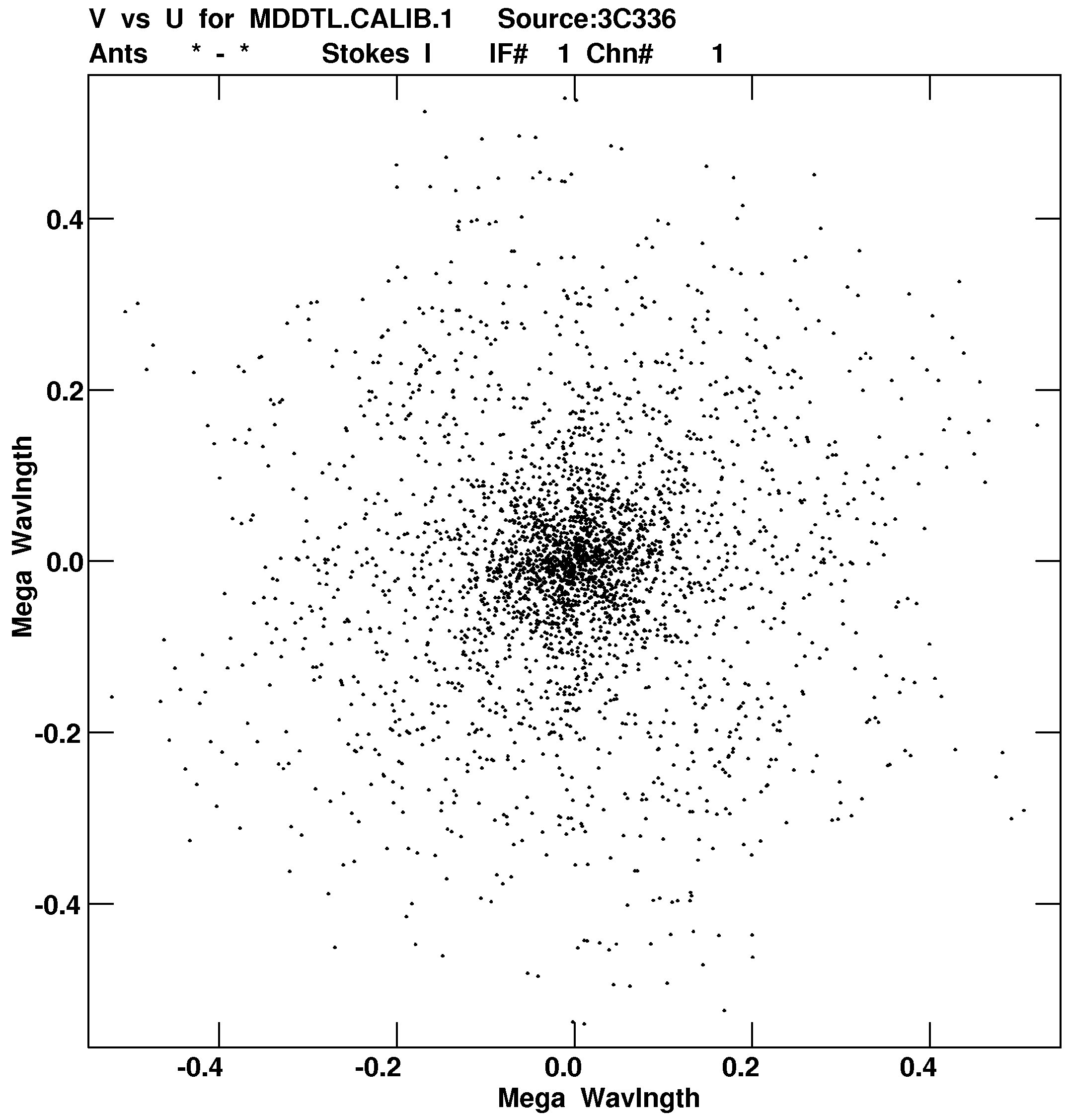
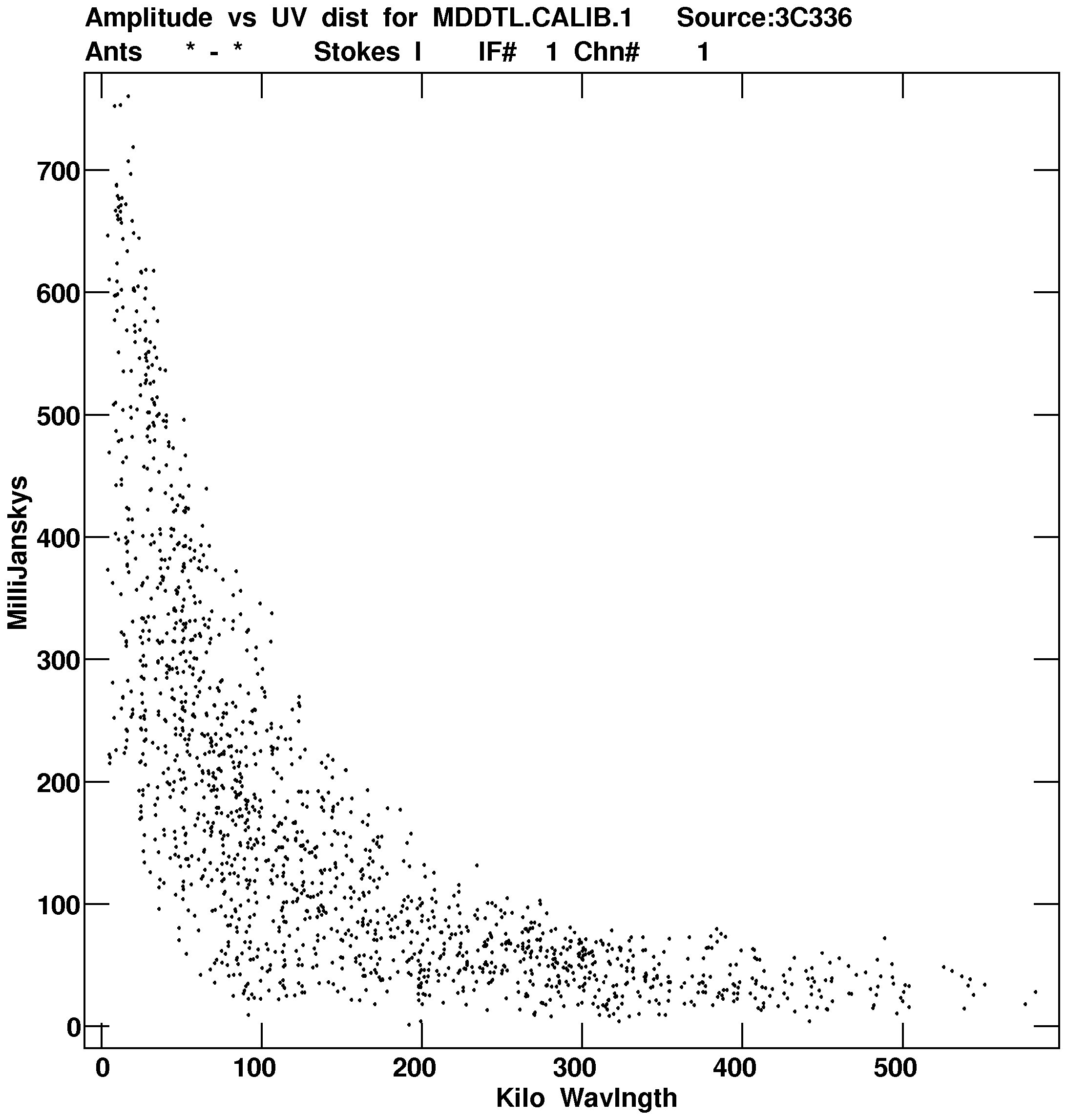
6.3.1 Plotting your visibility data

The most basic plot program for visibility data is called UVPLT. It allows you to select the x and y axes of the plot from real, imaginary, amplitude, log of amplitude, phase and weight of the visibility, time, hour angle, elevation, azimuth, and parallactic angle, and projected baseline length, position angle, u, v, w, frequency, spectral channel number, and baseline number. It offers all of the usual calibration and data selection options and it plots the selected points individually and/or in a controlled number of bins along the x axis. It can display multiple IFs and spectral channels at once, including averaging groups of spectral channels. It can also time average the data (SOLINT minutes) prior to plotting. For example, to plot calibrator phases as a function of time for all baselines to one antenna:

After UVPLT is running, or better, after it has finished:

There are several other tasks to plot your visibility data. VPLOT plots all of the parameters offered by UVPLT, but one baseline at a time with multiple baselines per page (i.e., per plot file) and multiple pages per execution. CLPLT is a similar task but restricted to plotting closure phases around baselines involving 3 antennas as a function of time. CAPLT is a similar task but restricted to plotting closure amplitudes around groups of 4 baselines as a function of time. All three of these can also plot a source model (based on Clean components) as well as the observations. In 31DEC22, task CLOSE can plot the rms of closure phase or amplitude as a function of spectral channel. ANBPL can create plots of amplitudes, phases, or weights converted to antenna-based quantities; this function is helpful in diagnosing problems with your data. For spectral-line users, POSSM plots visibility spectra averaged over selected baselines and time intervals. It can also plot various spectral tables (bandpass and others), as well as the Fourier transform of visibility spectra (the auto- and cross-correlation functions). POSSM can also plot other spectral tables (BD, PD, CP, PC, and PP). For VLBI users (primarily), FRPLT plots visibilities versus time or, more importantly, the fringe rate spectrum. To examine the statistical distribution of your data, try UVHGM which plots histograms showing the number of samples or weights versus a wide variety of parameters. Optionally, it will fit a Gaussian to the histogram and plot the result. The task UVIMG will grid visibility data into an image on a variety of axes, while the task UVHIM will make an image of a two-dimensional histogram of your uv data. All image display functions below may then be used to view the results. For example, if the axes of the histogram image are the real and imaginary parts of your data, then the image will demonstrate the amplitude and phase stability present (or missing) in your data.

Two tasks, new in 31DEC21, compute and then plot statistical information from calibrated autocorrelation data. VBRFI computes the statistics as a function of frequency and antenna and then prints them to a text file and, optionally, plots them. PLRFI can plot one or more of the text files written by VBRFI. As the names suggest, these are intended to describe the RFI environment of the antennas.

A number of visibility plotting and editing tasks offer the DO3COLOR option to separate multiple IFs, spectral channels, sources, times, and the like when plotted in the same plot area. Task PLOTC will make plots showing the colors used by such tasks with labels to assist in identifying which color goes with which data parameter. These plots may be saved as plot files and shown directly on the TV just as with all other plot tasks.

Three tasks allow you to examine selected portions of a uv data set statistically. UVRMS averages the selected data in SOLINT time intervals and then can plot the average values as a function of time and as a histogram. A variety of statistical parameters are computed and printed. SPRMS determines and plots the mean and standard deviation of the selected data as a function of spectral channel. Note that both tasks will combine data from multiple sources, baselines, etc. if so instructed. RIRMS computes statistics over the included visibility data and then prints a matrix over baselines of the real and imaginary parts separately. Histogram plots and plots over time may be generated.

Two plot programs actually convert visibility data to the image plane for plotting. Observers of point objects which might vary with time either intrinsically or by scintillation (e.g., stars, masers) might wish to try DFTPL, which plots the Fourier transform of the data shifted to a selected position as a function of time. Control over Stokes including polarization amplitude and popsition angle are available in 31DEC24. Tasks which save an image for later plotting include DFTIM which makes an image of such data as a function of frequency and time and ACIMG which makes a time and frequency image of autocorrelation data by antenna. VLBI spectral-line observers may need to use FRMAP, which performs imaging via fringe-rate inversion and plots the loci of possible source positions.

6.3.2 Plotting your image data

Image data may be drawn in a variety of ways including contours, grey or color levels, row tracing, and statistical. All plots are drawn with labeled tick marks although these may be suppressed with the LTYPE parameter. This LTYPE parameter is used to control the type of axis labels, the degree of extra labeling, the presence of the line giving the plot time and version, and also how metric scaling is done on the axis units. Read HELP LTYPE for details. For plots having significantly non-linear coordinate axes, e.g., wide-field images, it is sometimes useful to draw a full, non-linear coordinate grid rather than just short lines at the edges of the plot. Tasks like CNTR and even the verb TVLABEL offer this option; enter DOCIRC TRUE  C R.

Plot symbols (e.g., plus signs) may be drawn on the plots produced by CNTR, PCNTR, GREYS, KNTR and several of the other tasks mentioned below. In these tasks, the parameters which controls the plotting are STFACTOR, a scale factor for the symbols, and STVERS, a choice of the desired stars extension file. When using this option, there must be a table of “star” positions associated with the image being plotted. To create one, enter EXPLAIN STARS  C R to learn the format of the input data file and the parameters for the task. See also Appendix Z or your local equivalent for instructions on editing text files. A star file may also be created by MF2ST from a model fit file produced by task SAD (see §7.5.3 and §10.4.4). Tasks IMFIT, JMFIT, and SAD may now also produce “star” extension files directly.

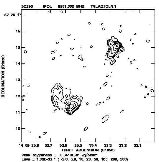
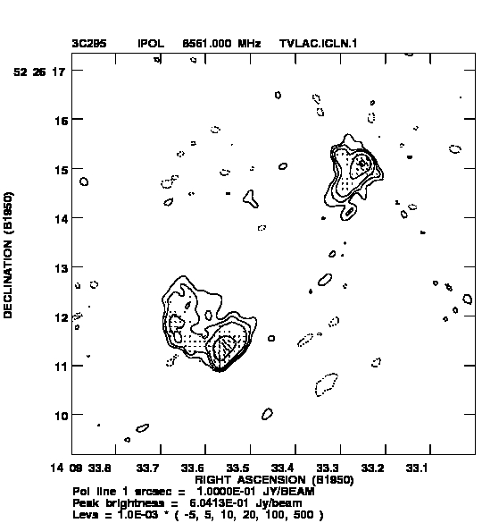
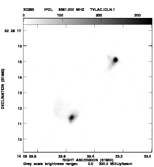
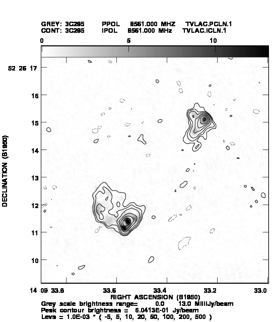
Example outputs of the following three tasks are given in Figure 6.2.

6.3.2.1 Contour and grey-scale plots

The most basic contour drawing task is CNTR. In addition to the usual image selection parameters, you may specify:

N.B., if you request more than one negative level with the LEVS input, you must use commas between the negative levels. Otherwise the minus sign(s) will be treated as subtraction symbols and the desired levels will be combined into a single negative level by the AIPS language processor. BLC and TRC can be initialized conveniently from the TV display using the cursor with the TVWIN instruction (see §6.4.4). Then check:

This generates a plot file as an extension to your image file, with the parameters you have just specified. Watch the  monitor (which, on some systems, is your terminal) to see the progress of this task. If the “number of records used” in the plot file is over 200, the contour plot will be messy (unless the field is also large). In this case, check that you have not inadvertently set PLEV or CLEV, for example, to unrealistically low values. Printing a large, messy plot file on the printer can take a considerable length of time and will inconvenience other users. Consider plotting directly on the TV first (DOTV = TRUE) to check on your selection of contours.

PCNTR plots polarization vectors on top of contours and/or grey-scales. You may make a polarized-intensity image and a polarization position-angle image from the Q and U images (see §7.1.2) or use the Q and U images themselves. Then:

Unless images 2 and 3 are of Q and U polarization, the lengths of the vectors are controlled by image 2 while the directions of them are controlled by image 3. Clearly this program can also be used for other combinations of images, so long as one of them represents an angle. PCNTR and following tasks have the option to draw an image of the Clean beam under control of adverb CBPLOT. Polarization vectors may be plotted with the color representing the angle. The value of POL3COL, if greater than zero, is that angle represented in pure red from 0 to 180 degrees. A color “spray” is plotted to calibrate the eye. To clarify the length scale of polarization vectors, a vector may be drawn in a box in an image corner under control of PVPLOT with the length of that vector in Jy/beam shown in a text line below the plot. The ability to plot multiple spectral planes in colored contour or polarization vectors was also added. The adverb CON3COL controls this function. The ability to select the colors of each contour level with RGBLEVS has been added. These color functions are displayed at the end of this chapter in the color pages.

GREYS creates a plot file of the grey-scale intensities in the first input image plane and, optionally, a contour representation of a second input image plane. Like the other grey-scale plotting tasks, GREYS can interpret a true-color (RGB) image cube in its “true” colors. Unlike the others, it can construct the true-color image from 3 separate image planes. A sample set of inputs could be:

When GREYS has finished, run LWPLA to view the plot file. Note that LWPLA has a variety of options which control the plotting and scaling of the grey-scale images without having to rerun GREYS. In this example case, you should remember to set FUNCTYPE = ’ ’ and DPARM = 0 (or at least the first 4 values to 0) in LWPLA to avoid additional scaling. You may wish to color the labeling, contours, and background with DOCOLOR=1 and PLCOLORS with LWPLA. The procedure TVCOLORS will set PLCOLORS to match the TV graphics-plane colors, DEFCOLOR will set PLCOLORS to the standard TV colors even in the absence of a TV display and OKCOLORS will set colors which work well with a white background, using less printer ink. See examples on the color pages at the end of this chapter.

There are two other contour drawing tasks which offer additional options. KNTR is able to draw multiple contour, polarization, and/or grey-scale images in a single plot file, primarily to show multiple planes of a spectral-line cube; see §8.5.4. KNTR uses a different, and probably superior, method of drawing the contour lines. It also can use color to represent different spectral channels and/or polarization angles or simply different colors for the different contour levels. CCNTR is virtually identical to CNTR except that it can draw extra symbols on the plot representing the locations and intensities of source model components found in CC (Clean component) or MF (model fit Gaussians from SAD, see §7.5.3 and §10.4.4).

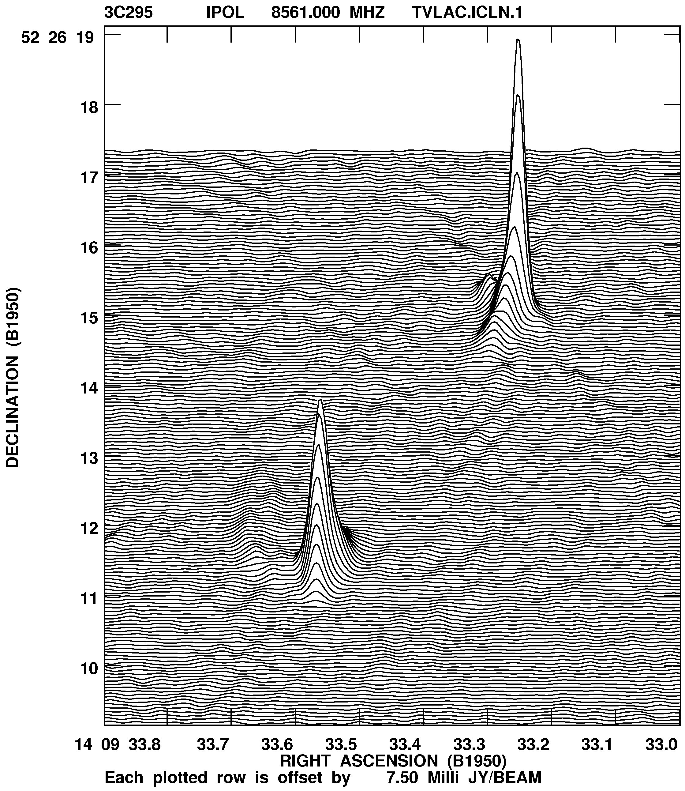
6.3.2.2 Row tracing plots

There are a number of tasks which plot rows directly. Two of these are for use with single image planes while others are more intended for use with, e.g., spectral-line data cubes transposed into velocity-ra-dec order. Of the former, PLROW is the simpler. It makes a plot file of all selected rows in an image plane. Each row is plotted as a slice offset a bit from the previous row. Low intensities which are “obscured” by foreground (i.e., lower row number) bright features are blanked to keep the plot readable. Example inputs would be:

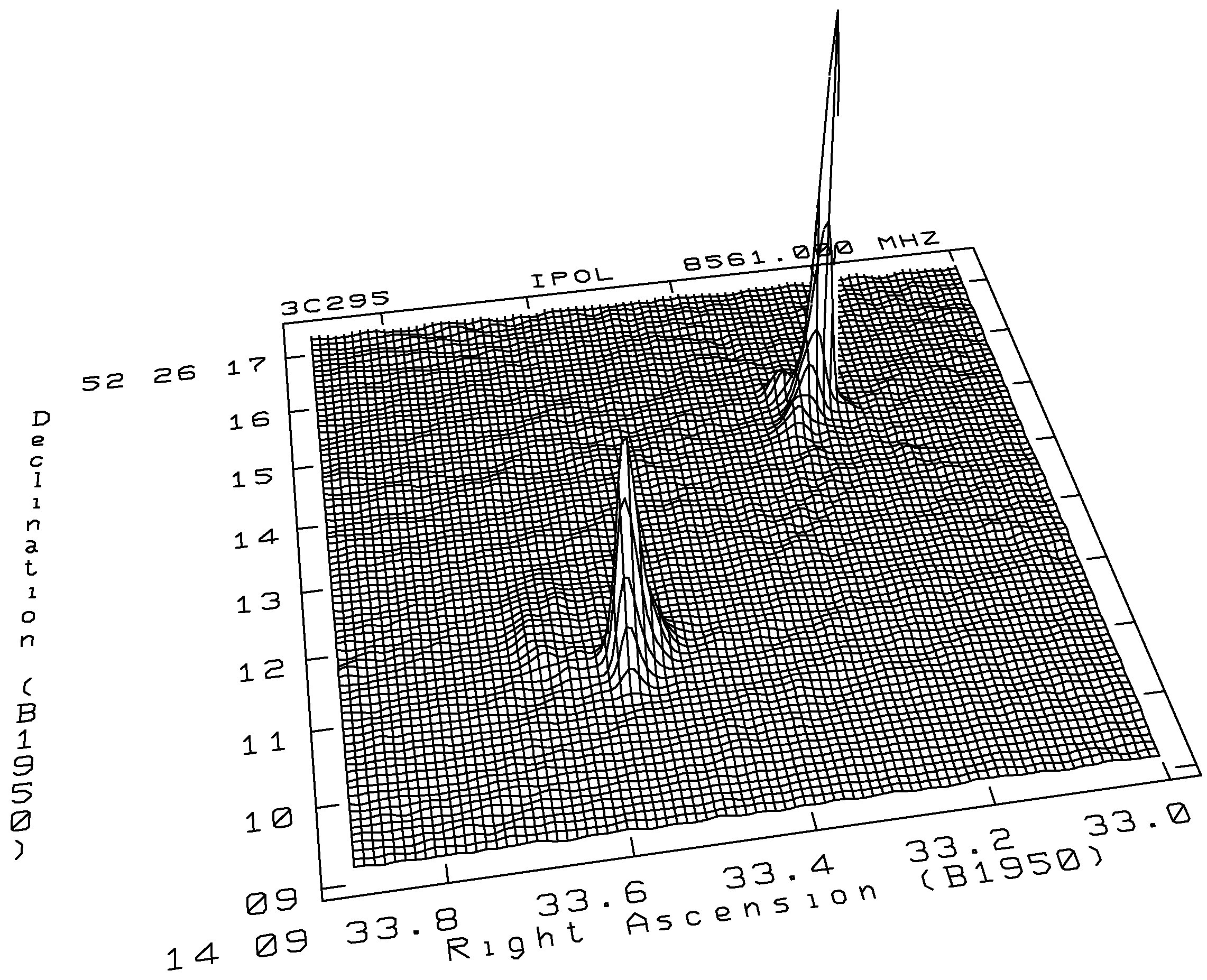
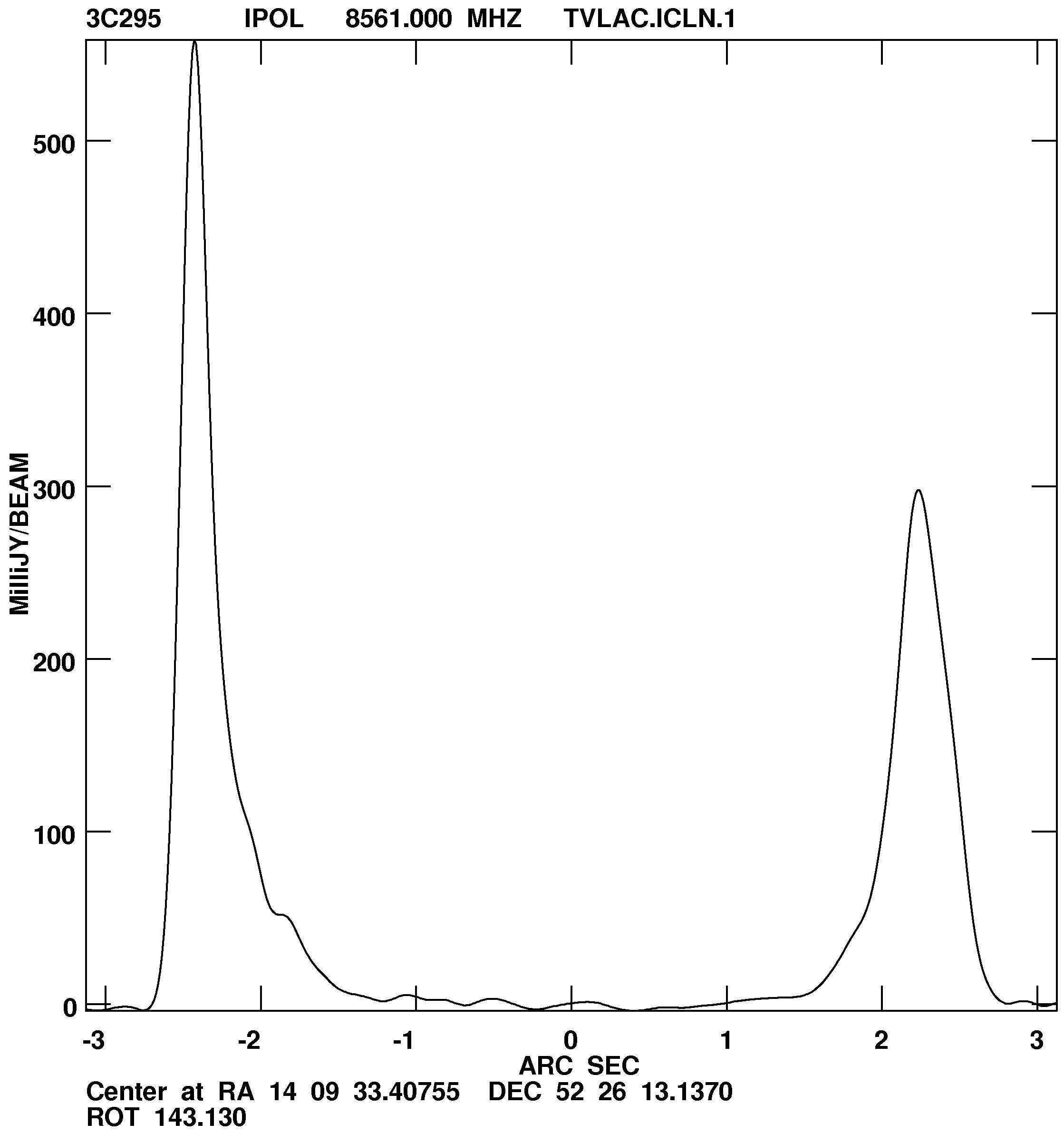
The plot files produced by PLROW are a simple, special case of those produced by PROFL. This task makes a plot file of a “wire-mesh” representation of an image plane complete with user-controlled viewing angles and correct perspective. Enter EXPLAIN PROFL  C R for a full description. Both of these tasks are especially useful where the signal-to-noise ratio is high and examples of them are given in Figure 6.3.2.2.

In Chapter 8 we discuss the computation and use of “slices,” one-dimensional profiles interpolated along any line in an image plane. Once a slice has been computed, it may be plotted by SL2PL on the TV or into a device-independent plot file.

Three other row-plotting tasks, PLCUB, ISPEC, and BLSUM, are designed primarily for spectral-line and other data “cubes” (see §8.5.4 and §8.6). PLCUB makes one or more plot files showing the intensities in each selected row. The row subplots are positioned in a matrix in the coordinates of the 2^nd and 3^rd axes of the cube. ISPEC averages circular or rectangular areas in each plane of a cube and plots the resulting spectrum. It can also save the output in a SLice file. RSPEC does the same except that it plots the robust or median absolute deviation (“MAD”) rms in each plane rather than the data. RSPEC has options to write out a signal-to-noise image and/or a text file of channel weights as well. BLSUM can plot spectra from irregular regions selected on the TV with a “blotch” algorithm.

6.3.2.3 Miscellaneous image plots

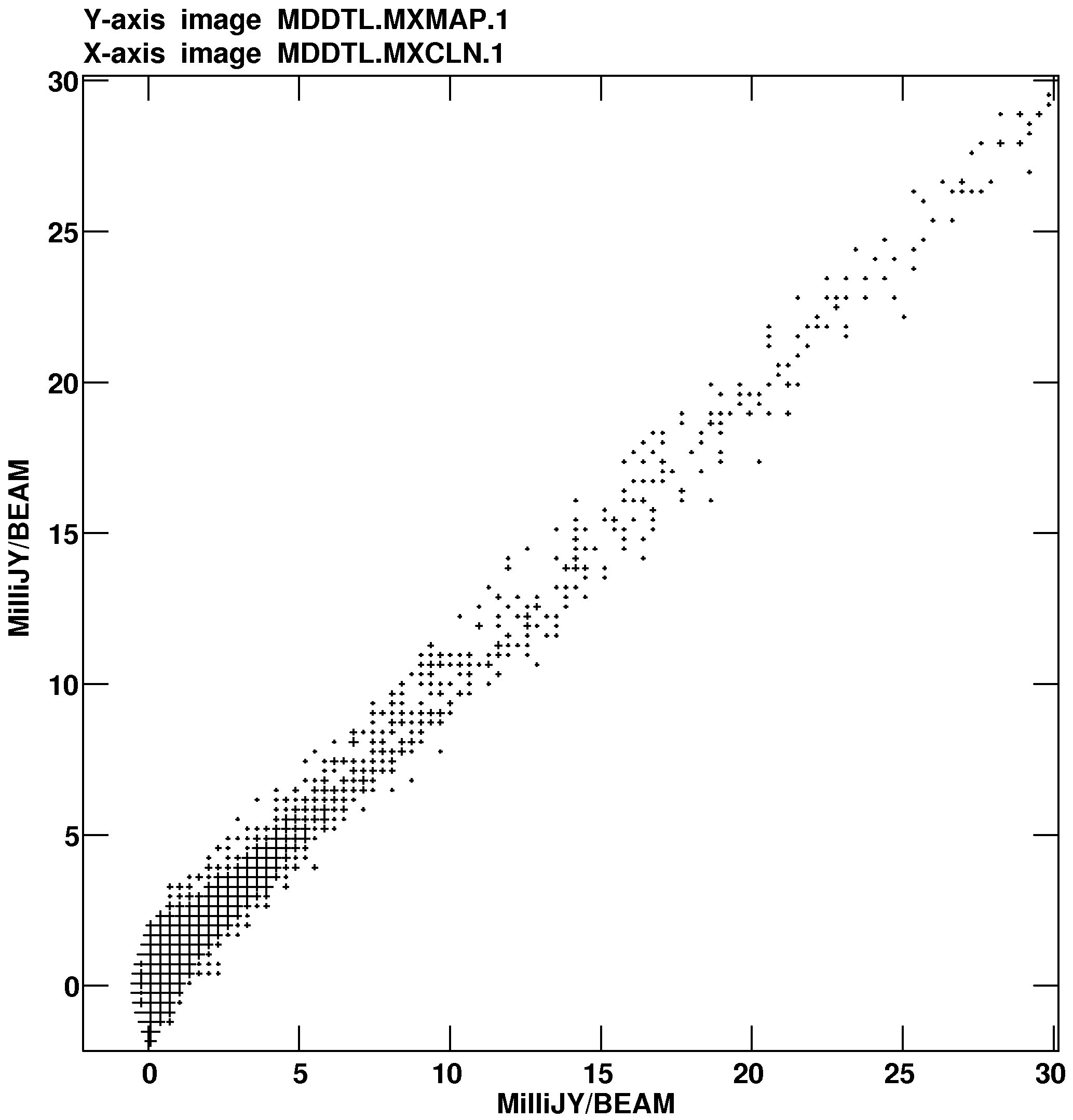
IMVIM allows a variety of image comparisons by plotting the pixel values of one image against the pixel values of another image. The special options include binning the values (and plotting symbols proportional to the number of samples in a bin) and shifting one of the images in x and/or y with respect to the other. The former reduces large scatter diagrams to more manageable sets of numbers while the latter allows cross-correlation functions to be developed.

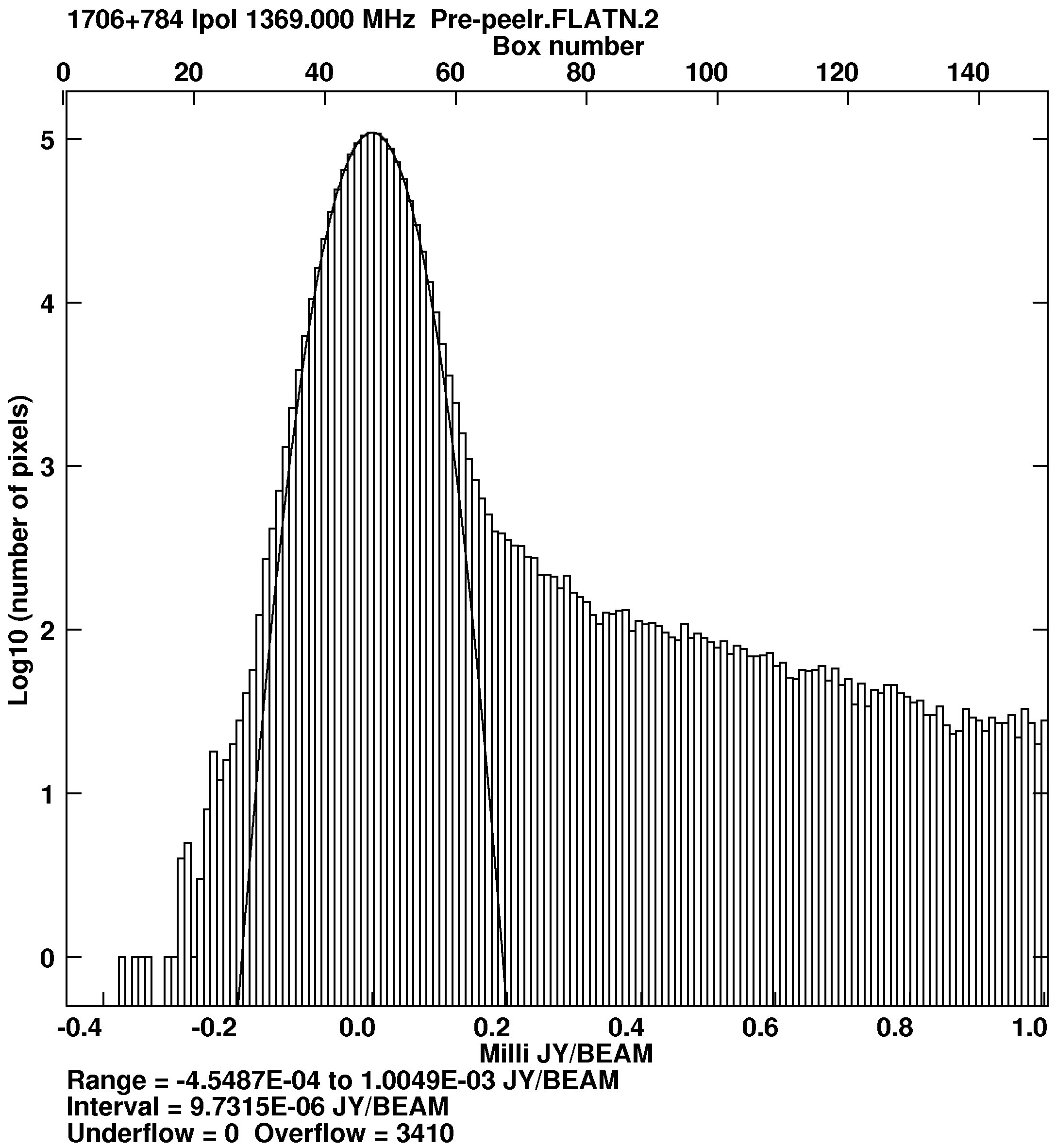
IMEAN prints the mean, rms, and extrema inside or OUTSIDE a user-specified window in an image. It also prints the intensity at, and rms of, the noise peak in the histogram and returns these values as adverbs to AIPS. It also returns an array in which TRIANGLE(i) is the brightness level above which there are i per cent of the image pixels. This is often useful in setting PIXRANGE for optical images. Optionally, IMEAN plots histograms of image intensities over the window using a user-specified number of summing cells over a user-specified range of intensities. Optionally, it also plots the fit to the noise peak on the user-specified histogram. An example of this is also shown in Figure 6.4.

6.3.3 Plotting your table data

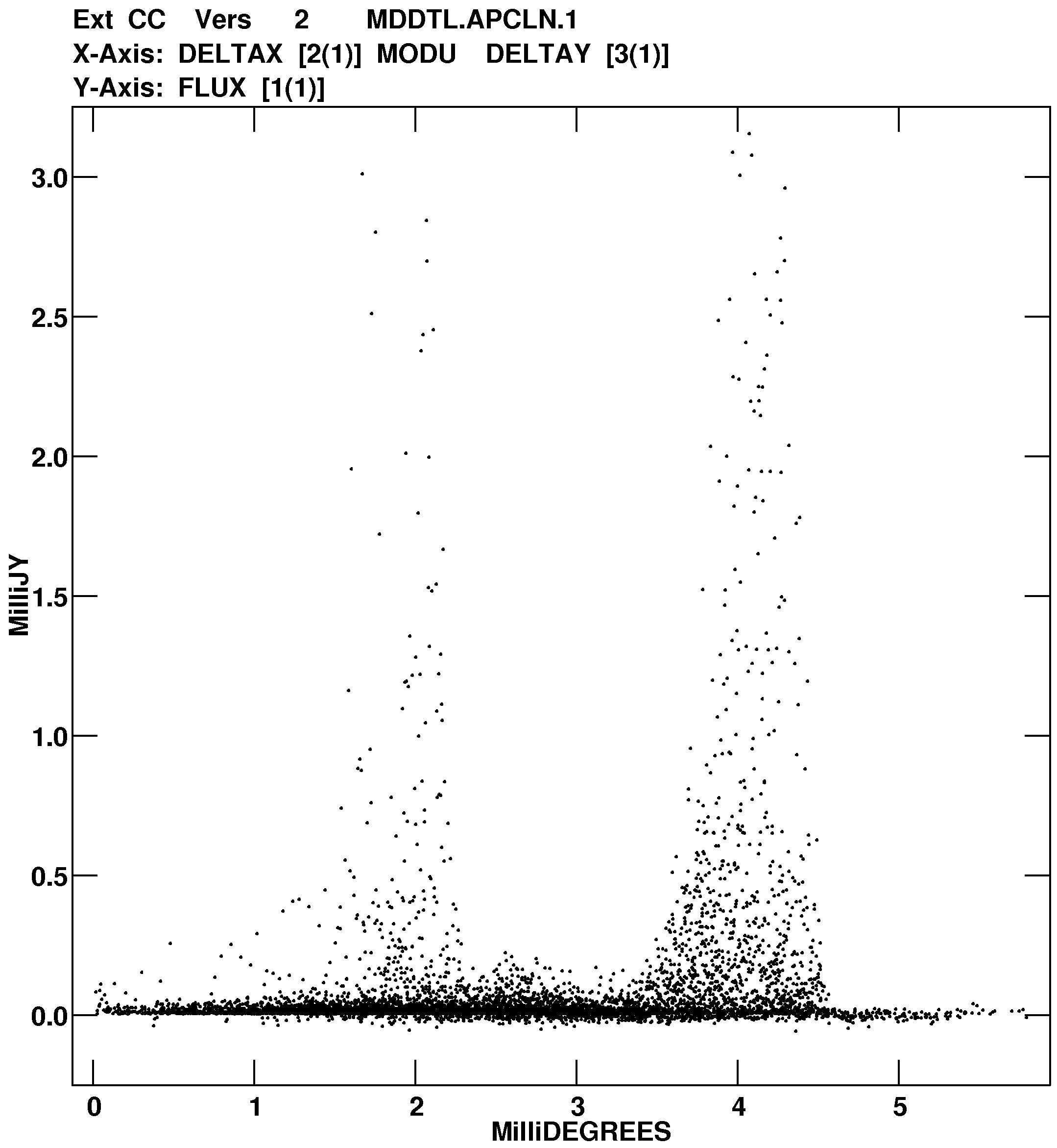
TAPLT is a very general task to plot information from  table extension files. It can plot a histogram of a function of the values in one or two columns of the table and it can plot a function of one or two columns against another function of another one or two columns. The latter can be summed or averaged in bins or have every point plotted. At first blush, the inputs seem rather complicated, but the results may well justify some effort to understand them. For example, to plot Clean component fluxes as a function of radius from the image center:

You may need to set the scaling with BPARM after seeing the preview plot in order, for example, to bring out the details in the low-level components.

There are a few tasks intended to make plotting specific kinds of tables rather easier. SNPLT plots calibration, solution, system temperature and EVLA SysPower tables for selected antennas as a function of time, antenna elevation, hour angle, azimuth, or sidereal time. It will make several plots per page (one antenna per plot) and multiple pages if needed, or you can plot the most discrepant value over all antennas in a single plot. In one execution, polarizations and IFs may be plotted on separate plots or together on the same plots, optionally separated by color. SNPLT also has the option to separate sources by color instead. You can also plot multiple parameter types in the same execution. SNBLP plots calibration solutions much like SNPLT, but on a baseline basis, to investigate exactly how the solutions affect the visibility data. SNIFS is similar to SNPLT but is intended to compare solutions at different IFs, plotting the IF on the x axis with a variety of binning options.

POSSM will plot bandpass tables when APARM(8) is set to 2. Values 3 – 10 plot bandpass-like tables from BLCHN (BD), PCAL (PD antenna polarization and CP source polarization), VLB pulse-cal (PC), and RLDIF (PP phase difference). POSSM can also do multiple plots per page with all the usual data selection adverbs. BPLOT also plots BP and the other similar tables, with multiple times for one antenna or multiple antennae for one time on each plot. Combined with difference and coloring options, this allows close comparison of bandpasses as functions of time or antenna. BLPLT makes a similar plot of the BL table written by BLCAL. BPEPL overplots multiple times within a BP table using color to separate times. It is similar to BPEDT without the interactivity. In 31DEC23, BPPLT plots selected portions of bandpass tables as a function of time in a manner similar to SNPLT. It is particularly useful when BPASS is used instead of CALIB to provide the gain calibration. WETHR plots the data in a WX weather table including parameters computed from those data such as relative humidity. FGPLT plots the times of selected flags from a flag table. PRTAN can plot antenna locations. New task TEPLT may be used to plot the ionospheric Faraday rotation and other parameters used by TECOR and written in a TE table.

6.3.4 Plotting miscellaneous information

There are a few other tasks which create plot files, but which do not fit into the categories above. The most general of these is PLOTR which can plot up to 30 sets of (x,y) points input from a text file with coloring options. Task PCHIS also reads a text file to produce a histogram plot of the values in any selected column of the file. CONPL is a task which plots  convolving functions (used by various uv-data gridding tasks such as IMAGR) and their Fourier transform, expected signal-to-noise ratio, or convolution with a user-specified Gaussian. IRING integrates an image in concentric annuli about the user-specified object center with specified major axis position angle and inclination. The results may be placed in a plot file for later display. GAL calculates the orientation and rotation curve parameters of a galaxy from an image of the predominant velocities. The observed rotation curve is plotted together with the fitted model curve. LOCIT fits antenna location corrections to SN tables; the residual phases may be plotted as a function of sample number.

There are several tasks which create RGB cubes for later display by tasks such as GREYS and KNTR. These include RGBMP which does a weighted sum of the planes of a data cube, HUINT which uses two images as hue and intensity to construct an RGB cube, and TVHUI which interactively uses three images as intensity, hue, and saturation to construct an RGB cube by a different algorithm. Task SCLIM will scale and clip image planes to be used as inputs to LAYER, which produces an RGB cube from the colored sum of up to 10 input image planes using a complicated and general algorithm.