7.6 Image analysis
Image analysis is a very broad subject covering essentially all that 


 does or would like to do
plus specialized programs designed to analyze a user’s particular image in the light of his favorite
astrophysical theories. provides some general programs to perform geometric conversions, image
filtering or enhancement, and model fitting and subtraction. These are the subjects of the following
sections. Specialized programs for spectral-line, VLBI, and single-dish data reduction are described in
Chapter 8, Chapter 9, and Chapter 10, respectively. Chapter 11 of Synthesis Imaging in Radio
Astronomy
covers the topic of image analysis in more detail.
does or would like to do
plus specialized programs designed to analyze a user’s particular image in the light of his favorite
astrophysical theories. provides some general programs to perform geometric conversions, image
filtering or enhancement, and model fitting and subtraction. These are the subjects of the following
sections. Specialized programs for spectral-line, VLBI, and single-dish data reduction are described in
Chapter 8, Chapter 9, and Chapter 10, respectively. Chapter 11 of Synthesis Imaging in Radio
Astronomy
covers the topic of image analysis in more detail.
7.6.1 Geometric conversions
The units of the geometry of an image are described in its header by the coordinate reference values, reference
pixels, axis increments, axis dimensions, and axis types. The types of coordinates (celestial, galactic, etc.) and the
type of tangent-plane projection (SIN from the VLA, TAN from optical telescopes, ARC from Schmidt telescopes,
NCP from the WSRT) are specified in the headers by character strings. See §6.1.2 and Memo No. 27
for details of these projections. A “geometric conversion” is an alteration of one or more of these geometry
parameters while maintaining the correctness of both the header and the image data. The tasks which do
this interpolate the data from the pixel positions in the input image to the desired pixel positions in the output
image.
The simplest geometric conversion is a re-gridding of the data with new axis increments and dimensions with no
change in the type of projection or coordinates. The task LGEOM performs this basic function and also allows rotation
of the image. One use of this task is to obtain smoother displays by re-gridding a sub-image onto a finer grid. To
rotate and blow up the inner portion of a 5122 image, enter:
> BLC 150 ; TRC 350 C R | to select only the inner portion of the image area. |
> IMSIZE 800 C R | to get an 8002 output image. This will allow the sub-image to
be blown up by a factor of 3 and rotated without having the
corners “falling” off the edges of the output image. |
> APARM 0 C R | to reset all parameters to defaults. |
> APARM(3) = 30 C R | to rotate the image 30∘ counterclockwise (East from North
usually). |
> APARM(4) = 3 C R | to blow up the scale (axis increments) by a factor of 3. |
> APARM(6) = 1 C R | to use cubic polynomial interpolation. |
> INP C R | to check the inputs. |
> GO C R | to run the program. |
LGEOM allows shifts of the image center, an additional scaling of the y axis relative to the x axis, and polynomial
interpolations of up to 7th order. OGEOM is similar to LGEOM, but handles blanked pixels in a manner that does not
increase the blanked area.
A much more general geometric transformation is performed by OHGEO and HGEOM, which convert one image into
the geometry of a second image. The type of projection, the axis increments, the rotation, and the coordinate
reference values and locations of one image are converted to those of a second image. One of these tasks
should be used before comparing images (with COMB, KNTR, PCNTR, BLANK, TVBLINK, etc.) made with
different geometries, i.e., radio and optical images in different types of projection or VLA images taken
with different phase reference positions. Use EXPLAIN OHGEO C R to obtain the details and useful
advice. SKYVE re-grids images from the Digital Sky Survey (optical DSS) into coordinates recognized by
.
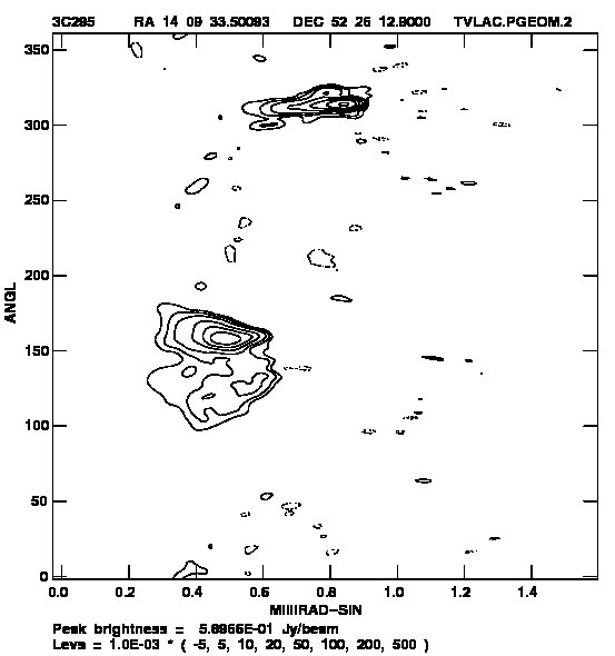
A potentially very powerful transformation is performed by PGEOM. In its basic mode, it converts between
rectangular and polar coordinates. An example of this operation is illustrated in Figure 7.1. However, PGEOM can
also “de-project” elliptical objects to correct for their inclination and “unwrap” spiral objects. Type EXPLAIN PGEOM
C R for information.
7.6.2 Mathematical operations on a single image
The task MATHS allows the user to do a mathematical operation on a single image on a pixel by pixel basis. Currently
supported mathematical operators are: SIN, COS, TAN, ASIN, ACOS, ATAN, LOG, LOGN, ALOG, EXP, POLY, POWR, and MOD.
An example of MATHS follows, in which the output image (OUT) is computed in terms of the natural logarithm of the
input image (IN) as follows: OUT = 4 + 2 × (log(3 × IN) - 1)
> INDI 0 ; MCAT C R | to help you find the catalog number of the input image. |
> INDI n ; GETN ctn C R | to specify the image, on disk n catalog slot ctn as the input. |
> OUTN ’xxxxx’ C R | to choose xxxxx as the name for the output image. |
> OUTC ’ccc’ C R | to choose ccc as the class for the output image. |
> OPCODE ’LOGN’ C R | to specify the operation to be performed (a natural logarithm). |
> CPARM 4 , 2 , 3 , -1 C R | to specify the coefficients. |
Undefined output pixels (in the current example, all pixels in the input image ≤ 0) are either blanked (CPARM(6)
≤ 0) or put to zero (CPARM(6) > 0). Type EXPLAIN MATHS C R for further information on the available operators and
the meaning of CPARM for any particular operator.
7.6.3 Primary beam correction
PBCOR allows correction for the attenuation due to the shape of the primary beam. Its use is straightforward:
> INDI 0 ; MCAT C R | to help you find the catalog number of the input image |
> INDI n ; GETN ctn C R | to select the input image from disk n catalog slot ctn. |
> OUTN ’xxxxx’ C R | to specify xxxxx for the name of the output image. |
> OUTC ’ccc’ C R | to specify ccc for the class of the output image |
> PBPARM 0 C R | to use the VLA, EVLA, ATCA, GMRT, or MeerKAT beam
parameters which are known for the particular receiver. |
> COORDIN 0 C R | to use the pointing position from the image header. |
The default behavior requested above uses the position in the header as the pointing position and uses the
empirically determined shape of the EVLA, VLA, MeerKAT, GMRT, or ATCA primary beam; PBCOR will scale the
primary beam shape according to the frequency provided in the image header and use the parameters associated
with the particular antenna feed. These defaults can be overridden by specifying particular values of COORDIN and
PBPARM. They beam parameters are frequency dependent within each band, so PBCOR determines the
beam value at the two tabulated frequencies nearest to the image frequency and then interpolates.
Gaussian and polynomial beam patterns have been added as options specified with OPCODE and APARM.
Also beam parameters for MeerKAT and GMRT are known to all tasks which correct for the primary
beam.
The task SPCOR may be used to apply corrections both for primary beam and for spectral index. The latter are based
on images of spectral index and spectral index curvature such as those used in IMAGR (§5.3.4.4). Such corrections
may be significant in Faraday-rotation synthesis (§7.2, §7.5.5).
An image of the primary beam may be generated with the task PATGN using OPCODE ’BEAM’ C R with other adverbs
to give the antenna type, frequency, cell size, image size, and, optionally, the parameters of the beam
shape.
7.6.4 Changing the resolution of an image
CCRES allows you to change the resolution of a Cleaned image by removing any Clean components in the image
and then restoring Clean components with your choice of resolution. The task may also be used to remove Clean
components to create a residual image or to restore Clean components to an existing residual image. CCRES allows
you to smooth or hyper-resolve your image. Unlike RSTOR, CCRES re-scales the residual image to put
it into units of Jy/beam for the new beam. This may be a superior way to image with a beam that
does not replicate the central portion of the dirty beam. IMAGR leaves the residual image in units of Jy
per dirty beam while restoring the Clean components in units of Jy per the Clean beam given in the
header.
Note that CCRES only changes the Clean components, not the residual image resolution. Furthermore, CCRES does
not take into account the varying resolutions of the many planes in an image cube. CONVL on the other hand, with
OPCODE ’GAUS’, will convolve both the Clean components and the residual to the requested resolution, taking into
account the change in input resolution as a function of frequency.
7.6.5 Filtering
For our purposes here, we can define “filtering” as applying an operator to an image in order to enhance some
aspects of the image. The operators can be linear or nonlinear and do, in general, destroy some of the information
content of the output image. As a result, users should be cautious about summing fluxes or fitting models in filtered
images. (Technically, these remarks can also be made about Clean and self-calibration.) However, filtered images
may bring out important aspects of the data and often make excellent, if unfamiliar-looking, displays of particular
aspects.
NINER produces an image by applying an operator to each cell of an image and its 8 nearest cells. The task offers
three nonlinear operators which enhance edges (regions of high gradient in any direction). It also offers linear
convolutions with a 3 × 3 kernel which can be provided by the user or chosen from a variety of built-in kernels.
Among the latter are kernels to enhance point sources and kernels to measure gradients in any of 8 directions. The
’SOBL’ edge-enhancement filter can bring out jets, wisps, and points in the data, while the gradient
convolutions produce images which resemble a landscape viewed from above with illumination at
some glancing angle (as when viewing the Moon). Both are very effective when displayed on the
TV or by the KNTR / LWPLA combination (see Figure 7.1). Enter EXPLAIN NINER C R for additional
information.
MWFLT, at present, applies any one of six non-linear, low-pass filters to the input image. Each filter is applied in a
user-specified window surrounding each input pixel. One of the operators is a “normalization” filter designed to
reduce the dynamic range required for the image while bringing out weaker features. Two of the
operators are a “min” and “max” within the window. When applied in succession, they produce a useful
low-pass filtered image (Rudnick, L. 2002, PASP, 114, 427). Other operators produce, at each pixel, the
weighted sum of the input and the median, the “alpha-trimmed” mean, or the alpha-trimmed mode
of the data in the window surrounding the pixel. These filters can be turned into high-pass filters
by subtracting the output of MWFLT from the input with COMB. Type EXPLAIN MWFLT C R for further
information.
Histogram equalization provides another form of non-linear filtering. HISEQ converts the intensities
of the full input image to make an output image with a nearly flat histogram. This magnifies small
differences in the heavily occupied parts of the histogram (usually noise) and diminishes large differences
in the less occupied parts (often real signal). TVHLD is an interactive task that loads an image to the
TV with histogram equalization and then allows the intensity range and method of computing the
histogram to be modified. It can write out at the end an equalized image in arbitrary (non-physical) units.
AHIST does an “adaptive” histogram equalization on each pixel using a rectangular window centered
on that pixel. This will magnify small differences in a more local sense, bringing out structures in
smooth areas of different brightness. SHADW generates a shadowed image as if a landscape having
elevation proportional to image value were illuminated by the Sun at a user-controlled angle. Although
these tasks magnify noise, they are likely to elucidate real structures in large areas of nearly constant
brightness.
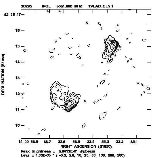
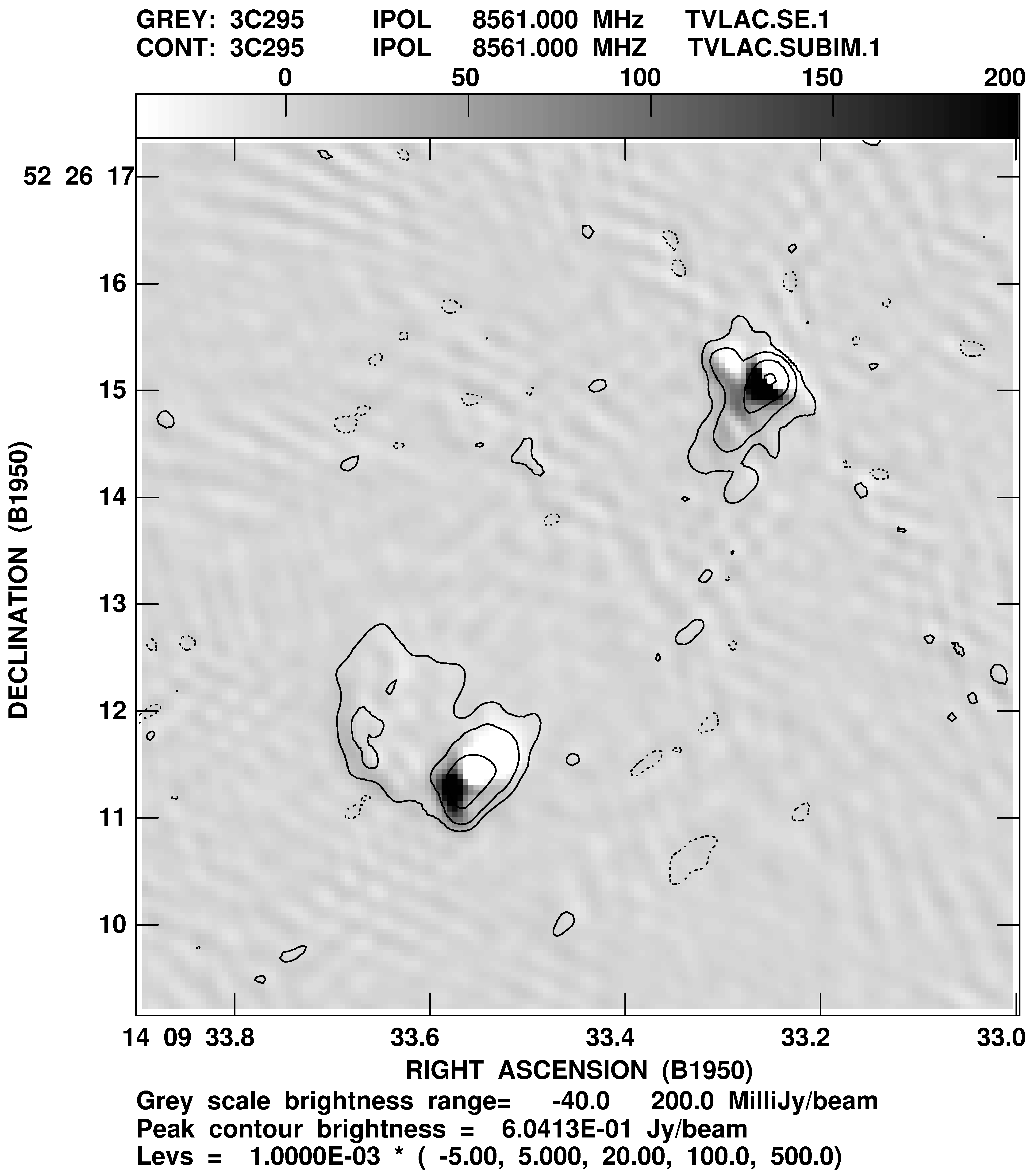
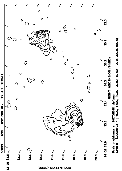 input image