The process of imaging in single-dish is a process of convolving the “randomly distributed” observations with some convolving function and then resampling the result on a regular image grid. Tasks SDGRD and SDIMG combine the data calibration, selection, projection, sorting, and gridding in one task capable of imaging all spectral channels into one output data “cube.” They are relatively easy to run, but selecting the correct input adverb values is more difficult. Choose SDGRD for most single-dish applications; SDIMG is very similar but can handle larger output images at the cost of making a sorted copy of the entire input data set (which can be very large). Type:
> DOCAL FALSE C R | to apply no calibration. |
> OPTYPE ’-GLS’ C R | to make the image on a “global sinusoidal” kind of projection. |
> APARM 0 C R | to use the observed right ascension and declination given in the header as the center of the image. For concatenated data sets, use APARM to specify a more appropriate center. |
> REWEIGHT 0, 0.05 C R | to have an “interpolated” or best-estimate image for output, cutting off any cells with convolved weight < 0.05 of the maximum convolved weight. |
> CELLSIZE c C R | to set the image cells to be c arc seconds on a side. |
> IMSIZE Nx , Ny C R | to make the image of each channel be Nx by Ny pixels centered on the coordinate selected by APARM. |
to select convolution function type 16 (a round Bessel function times Gaussian) with default parameters and 50 samples of the function per pixel. The default of 20 samples/cell is probably adequate. |
> INP C R | to review the inputs. |
> GO C R | to run the task. |
SDGRD begins by reading the data selecting only those samples which will fit fully on the image grid. It reports how many were read and how many selected. If you have made the image too small, with IMSIZE or CELLSIZE, then data will be discarded. Use PRTSD with a substantial XINC to determine the full spatial distribution of your data. It does not hurt to have the output image be a bit bigger than absolutely necessary. If you are uncertain about the parameters to use, try running SDGRD on a single channel to begin with since it will be much faster.
A number of these parameters require more discussion. REWEIGHT(1) selects the type of output image. The data are multiplied by their weights (which depend on the system temperature), convolved by the sampled convolving function and then summed at each image pixel. REWEIGHT(1) = 1 selects the result, which is not calibrated in any way since its scaling depends on the scaling of the data weights and the convolving function and on the distribution of data. While the program “grids” the actual data it also does the same process on the data replaced by 1.0. That result, the convolved weights may be obtained with REWEIGHT(1) = 2. The most meaningful image, which is obtained with REWEIGHT(1) = 0, is the ratio of the former to the latter. This is the interpolated or best-estimate image and will be similar to the convolved image in well-sampled regions except for having retained the calibration. REWEIGHT(1) = 3 tells SDGRD to compute an image of the expected noise (actually 1∕σ2) in the output image of type 0; see WTSUM below (§10.4.2) for its use.
REWEIGHT(2) controls which pixels are retained in the output image and which are blanked by specifying a cutoff as a fraction of the maximum convolved weight. It is important to blank pixels which are either simple extrapolations of single samples or, worse, extrapolations of only a couple noisy samples. In the latter case, it is possible to get very large image values. Thus, if the output is (W1D1 + W2D2)∕(W1 + W2) where the D’s are data and the W’s are convolved weights and if, say W1 = 0.1001,D1 = 1.0,W2 = -0.1000,D2 = -1.0, then the output would be 2001. Such large and erroneous values will be obvious, but will confuse software which must deal with the whole image and will also confuse people to whom you may show the image. In simple cases, in which all data have roughly the same data weights (system temperatures), setting REWEIGHT(2) = 0.2 or even more is probably wise. However, if some portions of the data have significantly lower weights than others, then you may have to set a lower value in order to keep the low-weight regions from being completely blanked.
The choices of CELLSIZE and the widths of the convolving function are related to the spatial resolution inherent in your data, i.e., to the single-dish beamwidth. If the pixels and function are too small, then data samples which are really from the same point in the sky will appear as if different in the output image. If, however, they are too large, then too much data will be smoothed together and spatial resolution will be lost. The latter may be desirable to improve signal-to-noise, but image smoothing can be done at a later stage as well. You may wish to experiment with these parameters, but it is usually good to start with a CELLSIZE about one-third of the beamwidth (fwhm) of your telescope. The default parameters (XPARMs) of all convolving functions may be used with this cell size. You may vary these parameters in units of cells or in units of arc seconds; enter HELP UVnTYPE C R to look at the parameters for type n (n = 1 through 6). If you give XTYPE = n + 10, then you get a round rather than square function which is perhaps better suited to this type of data. If you wish to change the cell size, but retain the same convolving function in angular measure on the sky, you may give XTYPE < 0 and specify the XPARMs in arc seconds rather than cells.
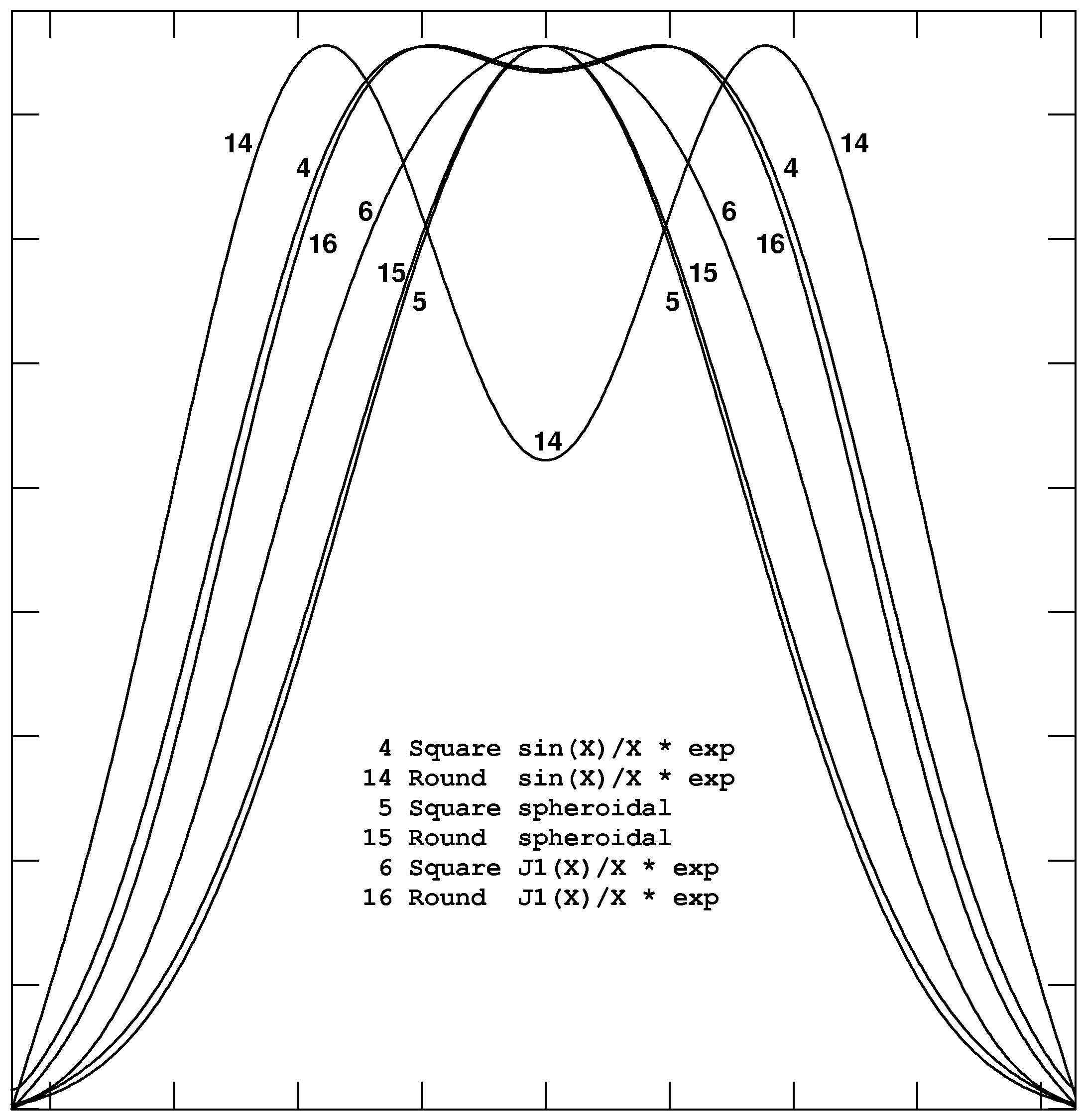
The choice of convolving function affects the noise levels and actual spatial resolution in the output image. In effect, the Fourier transform of the convolving function acts to modify the illumination pattern of the feed horn onto the aperture. Figure 10.4 shows slices through the Fourier transforms of six of the available convolving functions. The ideal function would be flat all the way across and then suddenly zero at the edges. Type 14 is the widest, but has a deep dip in the middle. This leaves out the center portion of the dish and illuminates the outer portions, effectively improving the spatial resolution of the image over that of the normal telescope, but with a noticeable loss of signal-to-noise ratio. The spheroidal functions, on the other hand, illuminate the center fully and leave out the outer portions. This degrades the spatial resolution, but noticeably improves the noise levels. Types 4 and 16 seem to be the best compromise. Type 16 is preferred since it is zero at the edges. Round functions require more computer memory than square ones, so type 4 would be preferred on computers with small memories.
Images may be built up from observations taken at significantly different times. The simplest way to do this is to concatenate the two “uv” data sets on disk with OTFUV or DBCON (§10.1.1.2) and then use SDGRD once to make the image. Some single-dish data sets are so large — or the time interval so great — that this is not practical. SDGRD combines observations taking into account the data weights which are based on the measured system temperatures. You can get the same weighted averaging in the image plane if you first compute a “weight” image and then use the task WTSUM to do the averaging. To get a weight image:
> REWEIGHT(1) 3 C R | to get the weight image which is proportional to 1∕σ2 expected from the actual gridding done on the data whose weights are assumed proportional to their 1∕σ2. |
to image a single channel when there is no channel-dependent data weights and flagging. |
> GO C R | to get the weight image. |
See §10.4.2 for details about WTSUM.
The construction of images from beam-switched on-the-fly continuum observations is more properly a research question than one of production software. Observers in this mode should be aware that the optimal methods of data reduction are probably not yet known and that the methods currently provided require the user to determine three critical correction parameters. In this mode, the telescope is moved in a raster of offsets in azimuth and elevation with respect to the central coordinate. The beam is switched rapidly from a “plus” position to a “minus” position at constant elevation. On the 12m, there are four plus samples and four minus samples taken each second, all taken while the telescope is being driven rapidly in azimuth at a constant (relative to the central source) elevation. In principle, each pair of plus and minus points contain the same instrumental bias but different celestial signals. It is then the job of the software to disentangle the time variable bias from the two beams’ estimates of the sky brightness.
A technique for doing the disentangling was first described by Emerson, Klein, and Haslam (Astronomy and Astrophysics, 76, 92–105, 1979). The plus and minus samples are differenced removing the instrumental bias and creating two images of the sky, one positive and one negative. Problems arise because the two images potentially can overlap and because, in the OTF mode of observing, the telescope positioning is not exactly along rows of the output image and the relative positioning of the plus and minus beams varies both due to the wobbles in the telescope pointing and due to the reversing of the direction of telescope movement. The Emerson et al. technique involves a convolution of each row in the differenced image with a function which is a set of positive and negative delta functions (or sin x x functions when the total beam throw is not an integer number of image cells). It turns out that the problem of image overlap is largely solved by this technique. Unfortunately, differences in the position of the plus and minus beam with respect to the source and to the image cells appear to limit the quality of the images produced with this technique.
The principal task used to produce images from data is called BSGRD. It makes two images from the two “uv” data sets written by OTFBS, gridding each sample at the coordinate at which it was observed (neglecting the throw but not the telescope movement between plus and minus). If the beam throw was not exactly along constant elevation, it then shifts the two images. Then it applies the Emerson et al. technique, fitting and removing baselines, differencing the two images, and convolving the difference image with an appropriate sin x x function. Finally, BSGRD re-grids the data from relative azimuth-elevation coordinates onto a grid in normal celestial coordinates. This task is a combination of four tasks, SDGRD described above to make the images, OGEOM to do the rotation correction, BSCOR to apply the Emerson et al. technique, and BSGEO to re-grid the data onto normal celestial coordinates.
To use BSGRD, type
to select the disk and catalog entry of the data set. Note that the class name is assumed to have a plus sign in the sixth character for the plus throw data set and a minus sign in that character for the minus throw data set. |
> DOCAL FALSE C R | to apply no calibration. |
> OPTYPE ’-GLS’ C R | to make the image on a “global sinusoidal” kind of projection. |
> APARM 0 C R | to use the observed right ascension and declination given in the header as the center of the image. For concatenated data sets, use APARM to specify a more appropriate center. |
> REWEIGHT 0, 0.05 C R | to have an “interpolated” or best-estimate image for output, cutting off any cells with convolved weight < 0.05 of the maximum convolved weight. |
> CELLSIZE c C R | to set the image cells to be c arc seconds on a side. |
> IMSIZE Nx , Ny C R | to make the image of each throw be Nx by Ny pixels centered on the coordinate selected by APARM. |
to select convolution function type 16 (a round Bessel function times Gaussian) with default parameters and 50 samples of the function per pixel. The same function is used in both convolutions. |
> FACTOR f C R | to multiply the recorded throw lengths by f in doing the Emerson et al. correction. |
> ROTATE ρ C R | to correct the throws for being ρ degrees off from horizontal. |
> DPARM 1, 1,x1,x2,x3,x4 C R | to specify that the two beams have the same relative amplitude and to give the pixel numbers to be used to fit baselines in both images. |
> ORDER 1 C R | to fit a slope as well as a constant in the horizontal baseline in each row. |
> INP C R | to review the inputs. |
> GO C R | to run the task. |
BSGRD takes three correction parameters which you must supply: the throw length error FACTOR, the throw angle error ROTATE, and the relative beam gain error DPARM(1). To estimate these, you will need data on a relatively strong point source. Use SDGRD to make an image of each throw of these data, setting ROTATE = 0 since rotation must be done later and setting ECHAN = 1 to eliminate the coordinate information which is confusing to MCUBE and used only by BSGEO. The tasks IMFIT and/or JMFIT (§7.5.2) may be useful in fitting the location and peak of the two beams. Since there is likely to be a significant offset from zero in these images, be sure to fit for the offset using a second component of CTYPE = 4. For reasons that are not clear, these tasks may not provide sufficiently accurate positions. Another approach then is to take the two images produced by SDGRD and then run OGEOM and BSCOR for a range of rotations and factors. Find the image that is most pleasing and put its parameters into BSGRD for the program source. Of course, it is not clear that these correction factors are constant with time or pointing, so this could all be bologna.
For example,
> APARM 0 C R | to do no shifts or re-scaling. |
> DOWAIT 1 C R | to wait for a task to finish before resuming AIPS. |
to produce 41 plus images each with a slightly different rotation. |
to produce 41 minus images each with a slightly different rotation. |
Then apply the Emerson et al. corrections to each of the 41 with
> FACTOR f C R | to multiply the recorded throw lengths by f in doing the Emerson et al. correction. Use 1.0 as an initial guess. |
> DPARM 1, 1,x1,x2,x3,x4 C R | to specify that the two beams have the same relative amplitude and to give the pixel numbers to be used to fit baselines in both images. The choice of the xn is significant. |
> ORDER 1 C R | to fit a slope as well as a constant in the horizontal baseline in each row. |
It is convenient to look at the images with tools such as TVMOVIE (§8.5.4) and KNTR (§10.4.5). To build the “cube”, use MCUBE as:
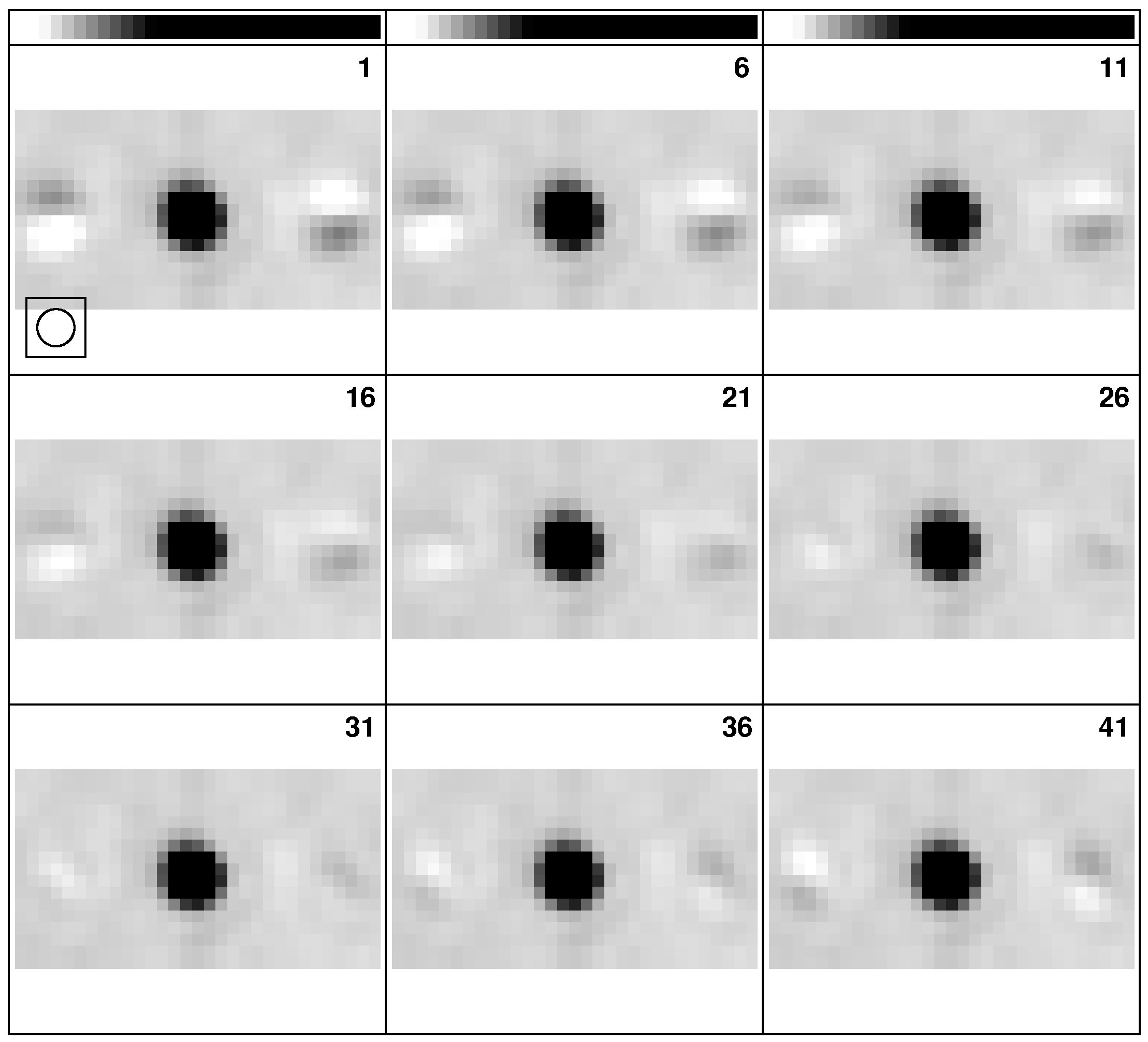
Examine the cube to find the “best” plane and use the rotation of that plane to run similar tests varying the throw length correction factor. One of these cubes, testing rotation, is illustrated in Figure 10.5.
The determination of throw length is similar:
to select the disk and catalog entry of the plus image at the best rotation. |
to select the disk and catalog entry of one of the corresponding rotated minus image. |
> DPARM 1, 1,x1,x2,x3,x4 C R | to specify that the two beams have the same relative amplitude and to give the pixel numbers to be used to fit baselines in both images. The choice of the xn is significant. |
> ORDER 1 C R | to fit a slope as well as a constant in the horizontal baseline in each row. |
> DOWAIT 1 C R | to run the task in wait mode. |
It is convenient to look at the images with tools such as TVMOVIE (§8.5.4) and KNTR (§10.4.5). To build the “cube”, use MCUBE as:
to select the disk and catalog entry of the first of the new corrected images. |
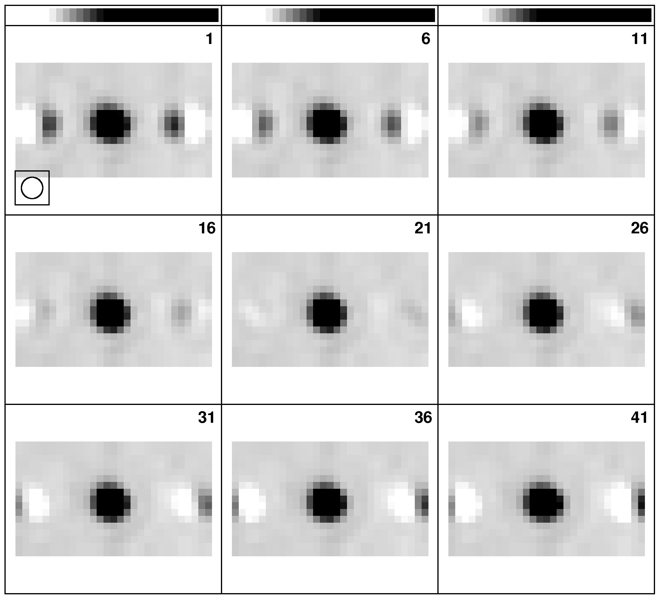
Examine the cube to find the “best” plane and use the scaling factor of that plane in later imaging. One of these cubes, testing throw length, is illustrated in Figure 10.6.
BSGRD is in fact a deconvolution algorithm to remove the plus-minus beam from the difference image. An experimental Clean algorithm has been made available in BSCLN. Although initial tests seemed promising, it appears to converge to the EKH solution after very many iterations and to have systematic problems before that point. The one-dimensional display task BSTST will allow you to evaluate and compare the two algorithms on model (one-dimensional) data.