O.1 The Historical VLA

The NRAO archive contains all of the data from the historical (or pre-EVLA) Very Large Array. These data are frequently mined for uses above and beyond those of the original observers. There is a new archive at https://data.nrao.edu; the old archive is no longer available. Log in at the above web address using your my.nrao.edu account and then select Show Search Inputs. This has all sorts of ways to find what you may desire. You may specify one or more of telescope, project code, date range, target name, target coordinates and search radius, observing band, or telescope configuration. You may submit your query and the tool will show you all data sets that match your specification. You may then request the data sets that you actually want and they will be downloaded to a publicly accessible disk area. All historical VLA data have been in the public domain for a long time, so no special permission should be needed. You will be notified when your data are available and told how to access them.

The old archive contained less well known content which is not available in the new archive. Instead the web site https:www.vla.nrao.edu/astro/nvas/ describes an archive of -processed legacy VLA data sets containing calibrated data and images. There is a description of this service and, at the left, buttons to connect to various web pages of informations and also a search tool.

For VLA data from the archive, use FILLM to read one or more disk files; see §O.1.1. The VLA format was changed on January 1, 1988, but all older data were translated and archived in the modern format. On July 1, 2007, the ModComps were replaced with modern computers and the format had an essential change made to it. Use FILLM to read data from both the ModComp and post-ModComp eras.

For VLA calibration, there are several useful procedures described in this chapter and Chapter 4. They are contained in the RUN file called VLAPROCS. Each of these procedures has an associated HELP file and inputs. Before any of these procedures can be used, this RUN file must be invoked with:

There is a “pipeline” procedure designed to do a preliminary calibration and imaging of ordinary VLA data sets. This provides a good first look at the data. Nonetheless, the results are still not likely to be of publishable quality. To run the pipeline, enter

See Appendix A for a simplified summary of data reduction suitable to data from the historic VLA. Much of the calibration of historic VLA data is similar to that of the modern EVLA, although the latter is fundamentally multi-channel and wide band. See Chapter 4 for a discussion of the steps used in calibrating all VLA data.

O.1.1 Reading from VLA archive files using FILLM

The NRAO Archive makes available, among other things, data from the EVLA, which began observing in January 2010, and from the old VLA which ceased observing a few days into 2010. To load data from the EVLA into  consult Chapter 4 for information about BDF2AIPS and other options. The following describes how to read old VLA data into .

The Archive now serves VLA data in the form of one or more “MOdComp” format disk files. To load these into , enter

In 31DEC21, FILLM first tries to open the file under the name in DATAIN. If that fails, it then tries the name in DATAIN with the file number appended as described above.

There are numerous adverbs including BAND, QUAL, CALCODE, VLAOBS. and VLAMODE to limit what data were loaded from magnetic tapes which could hold data from multiple projects. These adverbs still function, but are of little use today. Note that the values given above are illustrative and should not be copied verbatim in most cases.

Be careful when choosing the averaging time with CPARM(1). If you have a large data set, setting this time too low will make an unnecessarily large output file; this may waste disk space and slow the execution of subsequent programs. Setting it too high can, however, (1) smear bad data into good, limiting the ability to recognize and precisely remove bad data, (2) smear features of the image that are far from the phase center, and (3) limit the dynamic range that can be obtained using self-calibration. If you need a different (usually shorter) averaging time for the calibrator sources than for your program sources, use CPARM(10) to specify the averaging time for calibrators. See Lectures 12 and 13 in Synthesis Imaging in Radio Astronomy¹ for general guidance about the choice of averaging time given the size of the required field of view and the observing bandwidth.

CPARM(2) controls a number of mostly esoteric options. If your data include the Sun (see §O.1.8) or planets, you must set CPARM(2) = 16 to avoid having each scan on the moving source assigned a different name. The adverb DOWEIGHT = 1 has the same affect as CPARM(2) = 8 and both select the use of the nominal sensitivity to scale the data weights. When this is done, the weights will be 1∕σ² as they should for imaging, with σ in “Jy” in the same uncalibrated scale as the fringe visibilities. Having selected this option, you should apply any amplitude calibration to the weights as well as the visibilities. If you store the data in compressed form, only one weight may be retained with each sample. Any differences between polarizations and/or IFs in that sample will be lost. Uncompressed data require less CPU, but more real, to read but 2 to 3 times as much disk space to store.

CPARM(2)=2048 allows you to load data as correlation coefficients, which can be scaled to visibilities later with TYAPL (§O.1.3). CPARM(3) controls which on-line flags are applied by FILLM, which now always writes an OF table containing information about these flags. That information can be viewed with PRTOF and applied selectively to the data at a later time with OFLAG.

FILLM writes a weather (WX) table to the output file. At the same time, it uses “canned” VLA antenna gain curves and a balance of the current with a seasonal model weather data to estimate opacity and gain corrections to be written into the first calibration (CL) table. These functions are controlled by adverbs CALIN and BPARM and may be turned off, although the default is to make the corrections. In subsequent tasks, set DOCALIB = 1 to use these initial calibration data. If, for some reason, the data weights do not depend on the nominal sensitivity, use DOCALIB=100 to apply calibration.

Where possible, FILLM will try to place all data in one file. However, in many cases this is not possible. For instance so-called “channel 0” data from a spectral-line observation will be placed in a separate file from its associated line data. Similarly, scans which have differing numbers of frequency channels will also be placed into separate files. Another case is observations made in mode LP, i.e., one IF-pair is set to L band, the other to P band. In this case the two bands will be split into separate files. Yet another case arises when there are observations of different bandwidths. All of this should be relatively transparent to the user.

FILLM and many  tasks are able to handle multiple, logically different, frequencies within a multi-source data set. FILLM does this by assigning an FQ number to each observation and associating a line of information about that frequency in the FQ file associated with the data set. Users should note that this concept can become quite complicated and that not all tasks can handle it in full generality. In fact, most tasks can only process one FQ number at a time. Polarization calibration works only on one FQ at a time since the antenna file format allows for only one set of instrumental polarization parameters. Therefore, it is strongly advised that you fill continuum experiments which involve multiple frequencies into separate data sets. FILLM will separate bands automatically, but you will have to force any remaining separation. To do this, (a) use the QUAL adverb in FILLM, assuming that you have used separate qualifiers in OBSERVE for each frequency pair; (b) use the DPARM adverb array in FILLM to specify the desired frequencies precisely; or (c) use the UVCOP task to separate a multiple FQ data set into its constituent parts. Note that the first two options require multiple executions of FILLM, while the third option requires more disk space.

Spectral-line users and continuum observers using different frequencies in the same band should be aware of the FQ entry tolerance. Each frequency in a uv file will be assigned an FQ number as it is read from disk by FILLM. For spectral-line users, the observing frequency will normally change as a function of time due to Doppler tracking of the Earth’s rotation, or switching between sources or between spectral lines; in general, this will cause different scans to have different FQ numbers. FILLM assigns an FQ number to a scan based on the FQ tolerance adverb CPARM(7) which defines the maximum change of frequency allowed before a new FQ number is allocated. If CPARM(7) < 0, the the same FQ number is assigned to all data in spectral-line data sets. If CPARM(7) is positive, a scan’s will be assigned to an existing FQ number if

An example: if an observer observes the 1612, 1665 and 1667 MHz OH masers in VY CMa and NML Cygnus, then presumably he would like his data to have 3 FQ numbers, one associated with each OH transition. However, running FILLM with CPARM(7) set to 0 would produce 6 FQ numbers because the frequency difference between the masers in VY CMa and NML Cygnus is greater than the calculated tolerance of 160 kHz. Therefore, in order to ensure that only 3 FQ numbers are assigned, he should set CPARM(7) to 1000 kHz. Setting CPARM(7) < 0 would result in all data having the same FQ number, which is clearly undesirable.

For most continuum experiments the FQ number will be constant throughout the database. Normally any change in frequency should be given a new FQ number. To achieve this, FILLM treats CPARM(7) differently for continuum. If CPARM(7)≤ 0.0, then FILLM assumes a value of 100 kHz. A positive value of CPARM(7) is treated as a tolerance in kHz as in the spectral line case.

Note: If your uv database contains several frequency identifiers, you should go through the calibration steps for each FQ code separately.

FILLM can still read from magnetic tape. Set DATAIN to blanks, mount your tape (adverb INTAPE), index the tape with PRTTP, and use the adverbs to limit the data loaded to that portion of your project in which you are interested.

If FILLM is executing correctly, your message terminal will report the number of your observing program, the VLA archive format revision number, and then the names of the sources as they are found in the data files. Once FILLM has completed, you can find the database on disk using:

This should produce a listing such as:

You might then examine the header information for the disk data set by:

This should produce a listing like:

This header identifies the file as a multi-source file (Image=MULTI) with 2613887 floating-point visibilities in time-baseline (TB) order. There are two entries on the IF axis. These correspond to the old VLA’s “AC” and “BD” IF-pairs respectively. The description of the frequency (FREQ) axis shows that the first IF (“AC”) is at 8411 MHz and has 12.5 MHz bandwidth. The parameters of the second IF-pair (“BD”) are determined from the data in the FQ table file and cannot be read directly from this header; these values are shown in the ’SCAN’ listing from LISTR. The header shown above indicates that the data are in compressed format since the number of pixels on the COMPLEX axis is 1 and the WEIGHT and SCALE random parameters are not present. Uncompressed data does not use these random parameters and has 3 pixels on the COMPLEX axis.

The term “IF” can be confusing. At the VLA, IFs “A” and “C” correspond to right-hand and left-hand circularly polarized (RHC and LHC) signals, respectively, and are normally for the same frequency in an observing band. Such pairs, if at the same frequency, are considered to be one “IF” in . An observation which was made in spectral line mode “2AC” is considered at the VLA to have two “IFs” whereas within  this would be filled as one “IF” with two polarizations if they were both observed with the same frequency, the same number of channels, and the same channel separation. If these conditions do not hold, then they are filled into separate uv files, each with a single IF and a single polarization. The term “sub-array” is also confusing. At the VLA — and in task FILLM — sub-array means the subset of the 27 antennas actually used to observe your sources. (The historic VLA allowed up to 5 simultaneous sub-arrays in this sense.) In the rest of , sub-array refers to sets of antennas used together at the same time. If observations from separate times (e.g., separate array configurations) are concatenated into the same file, then  will regard the separate sets of antennas as different “sub-arrays” whether or not the same physical antennas occur within more than one of these sub-arrays.

Besides the main uv data file, this header listing shows that there are numerous “extension” files attached to the data. These are, in order, the history, antenna, index, source, frequency, calibration, system temperature, weather, and on-line flags tables. LISTR with OPTYPE=’SCAN’ provides a useful summary of the index, source, and frequency tables.

If your experiment contains data from several bands FILLM will place the data from each band in separate data sets. Also, if you observed with several sets of frequencies or bandwidths in a given observing run these will be assigned different FQ numbers by FILLM. You can determine which frequencies correspond to which FQ numbers from the ’SCAN’ listing provided by LISTR. Line data are divided into the “channel 0” (central 3∕4 of the of the observing band averaged) and the spectra. Data observed in the “LP” mode (or any other two-band mode) will be broken into separate data sets, one for each band.

O.1.2 Reading old spectral-line data

If your spectral-line data are in a VLA archive disk file, they should be read into  using FILLM, as described in §O.1.1. FILLM will fill a typical line observation into two files, a large one containing the line data only, and a smaller file containing the “channel-0” data. (Note that FILLM computes channel-0 from the line data rather than using the channel-0 provided by the on-line system.) The standard calibration and editing steps are performed on channel 0 and the results copied over to the line data set. You must be careful with the tolerance you allow FILLM to use in determining the FQ numbers. If you desire all of your data to have the same FQ number, so that you can calibrate it all in one pass, then set CPARM(7) in FILLM to an appropriately large value. If you wish to retain spectral-line autocorrelation data, you must set DOACOR to true.

By default for the VLA, the channel-0 data are generated by the vector average of the central 3/4 of the observing band. If this algorithm is not appropriate for your data, you may generate your own channel-0 data set by averaging only selected channels. You may now select different spectral channels in different IFs. To do this, use the task AVSPC:

You might find this necessary when observing neutral hydrogen at galactic velocities. Most calibrator sources have some absorption features at these frequencies.

O.1.3 Applying nominal sensitivities to historic VLA data

FILLM scales the correlation coefficients by the instantaneous measured “nominal sensitivities,” producing data approximately in deci-Jy. The VLA nominal sensitivities are stored in the TY table as “system temperatures” (T_sys). For calibration purposes, it is best to have the nominal sensitivities applied, but it may be better to use a clipped and/or time-smoothed version of those sensitivities. If you want to do this, load the T_sys data into the TY table with the highest time resolution possible by setting CPARM(9)=0 in FILLM. FILLM can also be told not to apply the nominal sensitivities and therefor produce correlation coefficients by setting CPARM(2)=2048, but this is not strictly necessary. In order to smooth and clip the TY table use the task TYSMO. If you have done editing such as QUACK, it may help to copy the data with UVCOP, applying your flag table not only to the visibilities but also to the TY table (UVCOPPRM(6)=3) before running TYSMO to remove questionable values at the start of scans. Alternatively, SNEDT will apply the data flags to the table allowing you to write a new, cleaned-up version of the table. Then a TY table may be applied (and/or removed) from a data set with TYAPL:

O.1.4 Calibrating historic VLA data

There are many similarities to the calibration of historic and modern VLA data. After reading in the data, you should with both run LISTR for the scan listing, PRTAN for the antenna layout information, and VLANT to correct antenna positions; see §4.2.2 and §4.3.1 for details. The general discussion on flagging (§4.3.10) applies to both types of data. However, with historic VLA data one does a purely continuum calibration and editing initially. If the observation is of spectral lines, the flag and calibration tables are copied to the line uv data file following the calibration of “channel 0.” Thus, the spectral editing tasks such as SPFLG, FTFLG, and RFLAG become useful only in the second half of spectral-line reductions. TVFLG (§O.1.6 below) is the preferred interactive editing task and editing with LISTR plus UVFLG (§O.1.5 below) is actually a reasonable option.

O.1.5 Editing with LISTR and UVFLG

Data may be flagged using task UVFLG based on listings from LISTR. To print out the scalar-averaged raw amplitude data for the calibrators, and their rms values, once per scan in a matrix format, the following inputs are suggested:

For unresolved calibrators, the VLA on-line gain settings normally produce roughly the same values in all rows and columns within each matrix. At L, C, X, and U bands, these values should be approximately 0.1 of the expected source flux densities. At P band, the factor is about 0.01. The factors for other bands are unspecified. Any rows or columns with consistently high or low values in either the amplitude or the rms matrices should be noted, as they probably indicate flaky antennas. In particular, you should look for

• In the amp-scalar averages, look for dead antennas, which are easily visible as rows or columns with small numbers. Rows or columns that differ by factors of two or so from the others are generally fine. Such deviations mean only that the on-line gains were not set entirely correctly.
• In the rms listings, look for discrepant high values. Almost all problems are antenna based and will be seen as a row or column. Factors of 2 too high are normally okay, while factors of 5 high are almost certainly indicative of serious trouble.

The next step is to locate the bad data more precisely. Suppose that you have found a bad row for antenna 3 in right circular polarization in IF 2 between times (d1, h1, m1, s1) and (d2, h2, m2, s2). You might then rerun LISTR with the following new inputs:

This produces a column listing on your terminal of the amplitude for baselines 1–2, 1–3 and 2–3 at every time stamp between the specified start and stop times. The ‘1–2” column provides a control for comparison with the two columns containing the suspicious antenna.

Note that “amp-scalar” averaging ignores phase entirely and is therefore not useful on weak sources, nor can it find jumps or other problems with the phases. To examine the data in a phase-sensitive way, repeat the above process, but set DPARM(2) = 0 rather than 1. Bad phases will show up as reduced amplitudes and increased rms’s.

Once bad data have been identified, they can be expunged using UVFLG. For example, if antenna 3 RR was bad for the full interval shown above, it could be deleted with

Continue the process until you have looked at all parts of the data set that seemed anomalous in the first matrix listing, then rerun that listing to be sure that the flagging has cleaned up the data set sufficiently. If there are lots of bad data, you may find that you have missed a few on the first pass. If you change your mind about a flagging entry, you can use UVFLG with OPCODE = ’UFLG’ to remove entries from the flag table. All adverbs of UVFLG are used when removing entries, so you may use REASON along with the channel, IF, source, et al. adverbs to select the entries to be removed. OPCODEs ’REAS’ and ’WILD’ may be used to undo an entry solely based on the REASON. If the table becomes hopelessly messed up, use EXTDEST to delete the flag table and start over or use a higher numbered flag table. The contents of the flag table may be examined at any time with the general task PRTAB and entries in it may also be removed with TABED and/or TAFLG. Two flag tables can be merged using TAPPE.

O.1.6 Editing with TVFLG

If your data are seriously corrupted, contain numerous baselines, and you like video games, TVFLG is the visibility editor of choice. The following discussion assumes that you have read §2.3.2 and are familiar with using the  TV display. The following inputs are suggested:

If you make multiple runs of TVFLG, it is important to make sure that the flagging table entries are all in one version of the FG table. The easiest way to ensure this is to set FLAGVER and OUTFGVER to 0 and keep it that way for all runs of TVFLG. If you make a mistake, two flag tables may be merged with the task TAPPE.

TVFLG begins by constructing a “master grid” file of all included data. This can be a long process if you include lots of data at once, even though a faster, large-memory method of gridding is now usually used. It is probably better to use the channel selection (including averaging channels with NCHAV), IF selection, source selection, and time range selection adverbs to build rather smaller master grid files and then to run TVFLG multiple times. It will work with all data included, allowing you to select interactively which data to edit at any one moment and allowing you to resume the editing as often as you like. But certain operations (such as undoing flags) have to read and process the entire grid, and will be slow if that grid is large. The master grid file is always cataloged (on IN2DISK with class TVFLGR), but is saved at the end of your session only if you set DOCAT = 1 (actually > 0) before starting the task. To resume TVFLG with a pre-existing master grid file, set the adverb IN2SEQ (and IN2DISK) to point at it. When resuming in this way, TVFLG ignores all of its data selection adverbs since they might result in a different master grid than the one it is going to use. If you wish to change any of the data selection parameters, e.g., channels, IFs, sources, times, or time averaging, then you must use a new master grid.

Kept with the master grid file is a special file of TVFLG flagging commands. This file is updated as soon as you enter a new flagging command, making the master grid and your long editing time virtually proof from power failures and other abrupt program terminations. These flagging commands are not entered into your actual uv data set’s flagging (FG) table until you exit from TVFLG and tell it to do so. During editing, TVFLG does not delete data from its master grid; it just marks the flagged data so that they will not be displayed. This allows you to undo editing as needed during your TVFLG session(s). When the flags are transferred to the main uv data set, however, the flagged data in the master grid are fully deleted since undoing the flags at that point has no further meaning. When you are done with a master grid file, be sure to delete it (with ZAP) since it is likely to occupy a significant amount of disk.

TVFLG keeps track of the source name associated with each row of data. When averaging to build the master grid and to build the displayed grids, TVFLG will not average data from different sources and will inform you that it has omitted data if it has had to do so for this reason. For multi-source files, the source name is displayed during the CURVALUE-like sections. However, the flagging table is prepared to flag all sources for the specified antennas, times, etc. or just the displayed source. If you are flagging two calibrator scans, you may wish to do all sources in between as well. Use the SWITCH SOURCE FLAG interactive option to make your selection before you create flagging commands. Similarly, you will need to decide whether flagging commands that you are about to prepare apply only to the displayed channel and/or IF, or to all possible channels and/or IFs. In particular, spectral-line observers often use TVFLG on the pseudo-continuum “channel-0” data set, but want the resulting flags to apply to all spectral channels when copied to the spectral-line data set. They should be careful to select all channels before generating any flagging commands. Each flagging command generated is applied to a list of Stokes parameters, which does not have to include the Stokes currently being displayed. When you begin TVFLG and whenever you switch displayed Stokes, you should use the ENTER STOKES FLAG option to select which Stokes are to be flagged by subsequent flagging commands.

If you get some of this wrong, you can use the UNDO FLAGS option in TVFLG if the flags have not yet been applied to the uv data set. Or you can use tasks UVFLG, TABED or TAFLG to correct errors written into the FG table of your multi-source uv data set. Flag tables are now used with both single- and multi-source data sets.

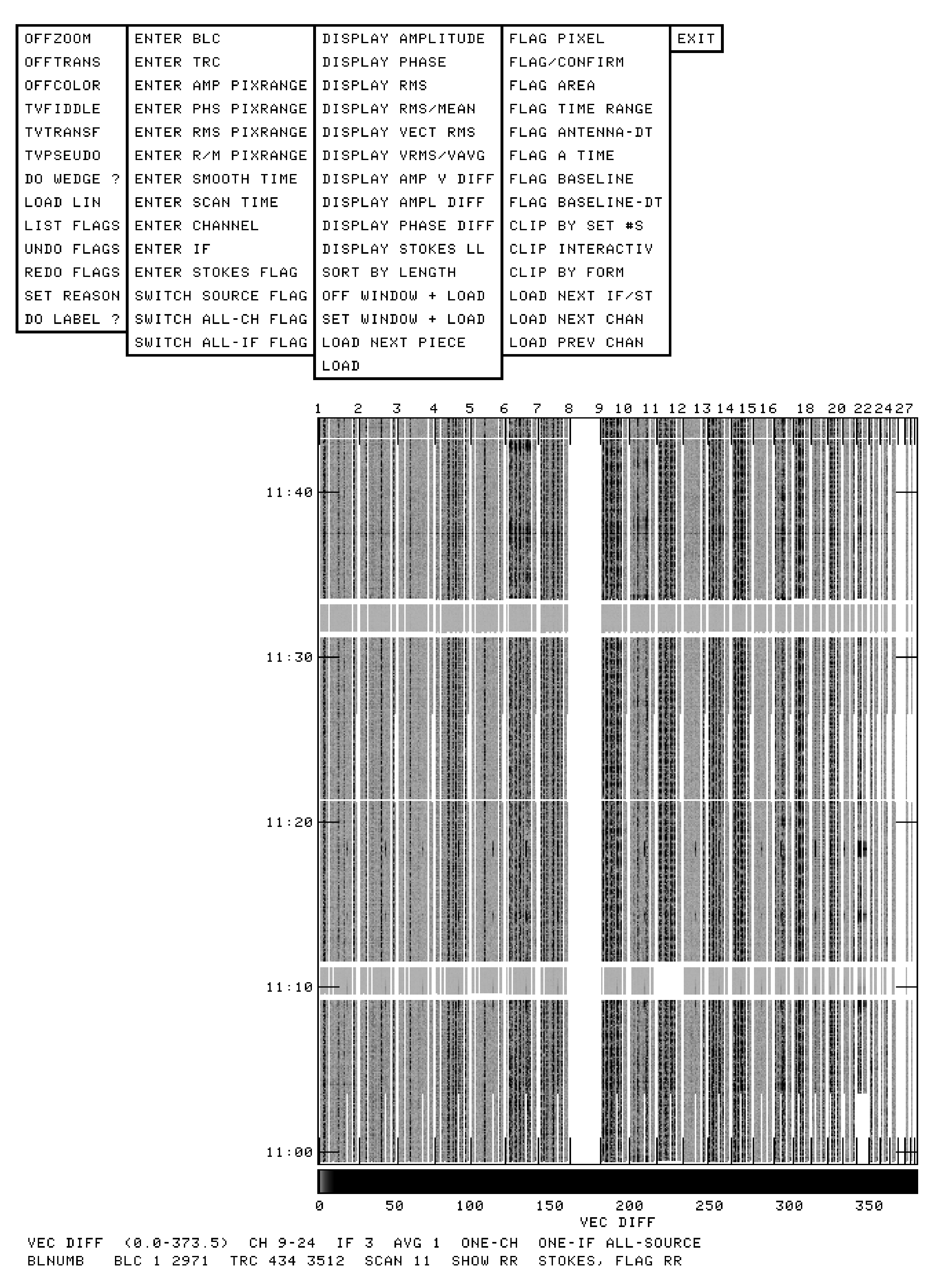
TVFLG displays the data, for a single IF, channel (average), and Stokes, as a grey-scale display with time increasing up the screen and baseline number increasing to the right. Thus baselines for the VLA run from left to right as 1–1, 1–2, 1–3, …, 2–2, 2–3, …, 27–27, 27–28, and 28–28. An input parameter (DPARM(3) = 1 allows you to create a master grid and display baselines both as, say 1–2 and 2–1. An interactive (switchable) option allows you to order the baselines from shortest to longest (ignoring projection effects) along the horizontal axis.

The interactive session is driven by a menu which is displayed on a graphics overlay of the TV display. An example of this full display is shown on the next page. Move the cursor to the desired operation (noting that the currently selected one is highlighted in a different color on many TVs) and press button A, B, or C to select the desired operation; pressing button D produces on-line help for the selected operation. The first (left-most column) of choices is:

Note: when a flag is undone, all cells in the master grid which were first flagged by that command are restored to use. Flag commands done after the one that was undone may also, however, have applied to some of those cells. To check this and correct any improperly un-flagged pixels, use the REDO FLAGS option. This option even re-does CLIP operations! After an UNDO or REDO FLAGS operation, the TV is automatically re-loaded if needed. Note that the UNDO operation is one that reads and writes the full master grid.

The load to the TV for all non-phase displays may be done with all standard transfer functions: LINear, LOG, SQRT, LOG2 (more extreme log). The menu shows the next one in the list (xxxx above) through which you may cycle. The TV is reloaded immediately when a new transfer function is selected.

Figure O.1: A display of a sample TV screen from TVFLG, made using the  task TVCPS to produce a negative black-and-white display. The TVFLG menu (in the boxes) is displayed in a graphics plane which is normally colored light green. The status line(s) at the bottom and optional axis labels are displayed in a graphics plane that is normally cyan in color. The data are grey scales in a TV memory and may be enhanced in black-and-white or pseudo-colored. The particular display chosen is the amplitude of the vector difference between the sample and a running vector average of samples surrounding it. This particular parameter is sensitive to both phase and amplitude problems and may save you the extra time of looking at phase and amplitude separately. It requires that there be data to average, but does not blur the flagging by the averaging interval (as the RMS method does). The visibility data are from the JVLA. All baselines are shown once only in baseline number order. Antenna 8 and 27 are missing for all times, while antennas 11 and 22 are missing for some times in the piece displayed here. The displayed data are the RR Stokes samples and have been windowed to exclude some times. Flag commands generated at the moment illustrated will flag all source names, one spectral channel (actually channels 9-24 averaged here), one IF, and Stokes RR only (from a 2-Stokes data set). The step wedge and labeling options have been selected.

Column 2 offers type-in controls of the TV display and controls of which data are to be flagged. In general, the master grid will be too large to display on the TV screen in its entirety. The program begins by loading every n^th baseline and time smoothing by m time intervals in order to fit the full image on the screen. However, you may select a sub-window in order to see the data in more detail. You may also control the range of intensities displayed (like the adverb PIXRANGE in TVLOD inside AIPS). The averaging time to smooth the data for the TV display may be chosen, as may the averaging time for the “scan average” used in some of the displays. Which correlators are to be flagged by the next flagging command may be typed in. All of the standard Stokes values, plus any 4-bit mask may be entered. The spectral channel and IF may be typed in. Flagging may be done only for the current channel and IF and source, or it may be done for all channels and/or IFs and/or sources. Note that these controls affect the next LOADs to the TV or the flagging commands prepared after the parameter is changed. When the menu of options is displayed at the top of the TV, the current selections are shown along the bottom. If some will change on the next load, they are shown with a trailing asterisk. Column 2 contains

The all-channel flag remains true if the input data set has only one channel and the all-IF flag remains true if the input data set has no more than one IF. If there are more than 2 IFs, the SWITCH ALL-IF FLAG cycles between flagging one IF, flagging a range of IFs, and flagging all IFs. When going to the range of IFs, it will ask you to enter the desired range.

An extra word should be said about the “scan average” to which reference was made above. This is used solely for displaying the difference of the data at time T and the average of the data at times near T. This average is computed with a “rolling buffer.” Thus, for a scan average time of 30 seconds and data at 10-second intervals, the average for a set of 7 points is as follows:

The third column of options is used to control which data are displayed and to cause the TV display to be updated. The master grid must be converted from complex to amplitude, phase, the rms of the amplitude, or the rms divided by the mean of the amplitude for display. It may also be converted to the amplitude of the vector difference between the current observation and the “scan average” as defined above or the absolute value of the difference in amplitude with the scalar-average amplitude or the absolute value of the difference in phase with the vector scan average. Furthermore, the baselines may be reordered in the TV display by their length rather than their numerical position. This column has the options:

SET WINDOW + LOAD is “smarter” than TVWINDOW and will not let you set a window larger than the basic image. Therefore, if you wish to include all pixels on some axis, move the TV cursor outside the image in that direction. The selected window will be shown. When there are more times than will fit on the TV screen at the current smoothing (averaging) time, the task divides the data up into overlapping time-range “pieces.” When it has done so, the LOAD LAST PIECE and LOAD NEXT PIECE menu items will appear. This lets you view one piece after the next, rotating through all pieces, to edit each time interval at full resolution. Note that a FLAG BASELINE will flag that baseline through all pieces.

The fourth column is used to select the type of flagging to be done. During flagging, a TV graphics plane is used to display the current pixel much like CURVALUE in AIPS. Buttons A and B do the flagging (except A switches corners for the area and time-range modes). Button C also does the flagging, but the program then returns to the main menu rather than prompting for more flagging selections. Button D exits back to the menu without doing any additional flagging. Another graphics plane is used to show the current area/time/baseline being flagged. All flagging commands can create zero, one, two, or more entries in the flagging list; hit button D at any time. There are also two clipping modes, an interactive one and one in which the user enters the clip limits from the terminal. In both, the current image computed for the TV (with user-set windows and data type, but not any other windows or alternate pixels etc. required to fit the image on the TV) is examined for pixels which fall outside the allowed intensity range. Flagging commands are prepared and the master file blanked for all such pixels. In the interactive mode, buttons A and B switch between setting the lower and upper clip limits, button C causes the clipping to occur followed by a return to the main menu, and button D exits to the menu with no flagging. The options are

The CLIP BY FORM operation allows you to apply a clipping method already used on one channel/IF to other channels and/or IFs. It asks for a command number (use LIST FLAGS to find it) and applies its display type (amp, phase, rms, rms/mean, differences), averaging and scan intervals and clip levels to a range of channels, IFs and Stokes (as entered from the terminal). To terminate the operation, doing nothing, enter a letter instead of one of the requested channel or IF numbers. To omit a Stokes, reply, if requested for a flag pattern, with a blank line. You may watch the operation being carried out on the TV as it proceeds.

The right-most column has only the option:

Before the flags are entered in the data, TVFLG asks you whether or not you actually wish to do this. You must respond yes or no. Note that, if the master grid is to remain cataloged, there is no need to enter the flagging commands every time you decide to exit the program for a while. In fact, if you do not enter the commands, you can still undo them later, giving you a reason not to enter them in the main uv data set too hastily.

The two most useful data modes for editing are probably amplitude and amplitude of the vector difference. The former is useful for spotting bad data over longer time intervals, such as whole scans. The latter is excellent for detecting short excursions from the norm. For editing uncalibrated data, rms of two time intervals is useful, but the rms modes require data to be averaged (inside TVFLG) and therefore reduce the time resolution accuracy of the flagging. If you edit by phase, consider using the pseudo-coloration scheme that is circular in color (option TVPSEUDO followed by button B) since your phases are also circular.

Using TVFLG on a workstation requires you to plan the real estate of your screen. We suggest that you place your message server window and your input window side-by-side at the bottom of the screen. Then put the TV window above them, occupying the upper 70–90% of the screen area. (Use your window manager’s tools to move and stretch the TV window to fill this area.) Instructions and informative, warning and error messages will appear in the message server window. Prompts for data entry (and your data entry) appear in the input window. Remember to move the workstation cursor into the input window to enter data (such as IF, channel, antenna numbers, and the like) and then to move the cursor back into the TV area to select options, mark regions to be flagged, adjust enhancements, and so on.

O.1.7 Spectral-line calibration

The calibration of spectral-line data is very similar to that of continuum data with the exception that the antenna gains have to be determined and corrected as a function of frequency as well as time. The model used by  is to determine the antenna gains as a function of time using a pseudo-continuum (“channel-0”) form of the data. Then the complex spectral response function (“bandpass”) is determined from observations of one or more strong continuum sources at or near the same frequency as the line observation. In general, the channel-0 data are calibrated using the recipes in the previous sections of this chapter. The sub-sections below are designed to bring out the few areas in which spectral-line calibration differs from continuum.

O.1.7.1 Spectral-line aspects of SETJY

The LISTR output with OPTYPE = ’SCAN’ will show information from the source table including spectral-line parameters. VLA data from FILLM are normally supplied with adequate information regarding the source velocity, line rest frequency, and velocity reference (radio versus optical, LSR versus barycentric). However, data from the EVLA and other telescopes may be missing these parameters. SETJY must then be used to fill in the needed values. An OPTYPE=’VCAL’ option computes the velocity of the reference channel from first principles. It is recommended over inaccurate guesses of adverb values in other SETJY OPTYPEs. It may be run over all sources after the rest frequencies and velocity reference information has been filled in.

O.1.7.2 Editing the spectral data

You should follow the steps outlined in §4.3.5 to edit the calibrator data using the channel-0 data set. Even though channel-0 data is continuum, be careful to have TVFLG and UVFLG generate the flagging commands for all channels, not just channel 1. Then, copy the resulting FG table to the line file. Use TACOP:

Specifying the “ALL-CH” setting in TVFLG and specifying BCHAN 1 ; ECHAN 0  C R in UVFLG cause all channels to be flagged when the FG table is copied to the line data set.

Spectral-line observers should also use SPFLG (§10.2.2) to examine and, perhaps, to edit their data. This task is very similar to TVFLG described in §O.1.6, but SPFLG displays spectral channels for all IFs on the horizontal axis, one baseline at a time. If you have a large number of baselines, as with the VLA, then you should examine a few of the baselines to check for interference, absorption (or emission) in your calibrator sources, and other frequency-dependent effects. Use the ANTENNAS and BASELINE adverbs to limit the displays to a few short spacings and one or two longer ones as well. If there are serious frequency-dependent effects in your calibrators, use SPFLG and UVFLG to delete them. (You might wish to delete the FG table with EXTDEST to begin all over again.) Then use AVSPC to build a new channel-0 data set and repeat the continuum editing. Note that you should not copy the FG table from the spectral-line data set to the new continuum one. The reason for this is the confusion over the term “channel.” If you have flagged channel 1, but not all channels, in the spectral-line data set — a very common occurrence — then a copied FG table would flag all of the continuum data since it has only one “channel.” When you have flagged the channel-0 data set, you can merge the new flags back into the spectral-line FG table with task TABED.

If the channel-0 data set is meaningful for your program sources, you might consider doing a first-pass editing of them along with your calibrators before copying the FG table back to the line data set. If your program sources contain significant continuum emission, then this is a reasonable operation to perform. If they do not, then the standard channel-0 data set is not useful for editing program sources. You can use SPFLG to edit all channels, or if the signal is strong in a few channels, you could run TVFLG on those channels from the spectral-line data set or average those with the BCHAN, ECHAN, and NCHAV adverbs.

O.1.7.3 Calibrating the spectral data

The channel-0 data set should be calibrated as described above for continuum data (§4.3.5 and §4.3.10). When you are satisfied with your results, you should copy the relevant CL table over to the line data set with TACOP:

If you copy SN, TY, or SY tables, you may apply a flagging table to the table values.

Then one runs BPASS on the bandpass calibration source(s). This is the same process as for the modern VLA; see §4.3.8 for details.

At this point it is often useful to examine your fully calibrated data using POSSM:

If you have multiple FQ entries in your data set, you should repeat the calibration for each additional FQ entry. Bookkeeping is simplified if you eliminate all extant SN tables before calibrating the data associated with each frequency identifier. However, it is not essential to do this.

O.1.8 Solar data calibration for the historic VLA

The calibration of solar uv data differs from normal continuum and spectral-line calibration in one critical respect: the system temperature correction to the visibility data is applied by the observer in . See Lecture 21 in Synthesis Imaging in Radio Astronomy for a discussion of the system temperature correction as it applies to VLA solar visibility data. The system temperature correction is embodied in a quantity referred to as the “nominal sensitivity,” an antenna-based numerical factor normally applied in real time to the scaled correlation coefficients before they are written to the VLA archive. With the exception of X and L band, only a handful of VLA antennas are equipped with so-called “solar CALs.” The nominal sensitivity is only computed for those antennas so-equipped, namely (for the old VLA) antennas 5, 11, 12, and 18 (at K, U,and C bands) and antennas 7, 12, 21, and 27 (at P band). The system-temperature correction for those antennas without solar CALs must, therefore, be bootstrapped from those antennas which do have solar CALS. This is accomplished through two tasks for the old VLA and two other tasks for the new VLA.. For the old VLA, FILLM fills the uncalibrated visibility data to disk and places the nominal sensitivities in a TY extension table. Then, SOLCL applies the nominal sensitivities to calibration parameters in the CL table. For the new VLA, BDF2AIPS reads the data in, writing a SysPower (SY) and CalDevice (CD) table. Then SYSOL applies the gain and weight corrections. See §4.1.1 and §4.3.15.

O.1.8.1 Reading solar data from the VLA archive

To load a solar uv-data file to disk from an old VLA archive data set follow the general instructions given above (§O.1.1 and §O.1.2) with the following additions:

If your experiment involved observing active solar phenomena, (e.g., flares), you may wish to update the system-temperature correction every integration time. For example, if you observed a flare with an integration time τ = 1.67 seconds, choose

Loading an entire solar uv-data set to disk with the minimum integration time results in large disk files which make all subsequent programs take a longer time to run. By modern standards, historic VLA data sets are relatively small, so the following may no longer be necessary. A useful strategy is to load the data with relatively low time resolution (20–30 seconds for observations of active solar phenomena) and to proceed with the usual continuum data calibration, deferring the system temperature correction. When a satisfactory calibration is obtained, the relevant SN table may be saved using TASAV. (Note that you must save the SN table, before running CLCAL rather than the final CL table.) Then run CLCAL and inspect the data for interesting periods of activity — try UVPLT with BPARM = 11, 1 for plots of amplitude versus time or TVFLG, displaying amplitudes as a function of baseline length and time. Use FILLM to load the relevant time ranges of solar uv data to disk with no averaging. The saved SN table is then copied to each high-time resolution data set. Assess, and possibly edit, the nominal sensitivities (§O.1.8.2) and then apply the system-temperature corrections (§O.1.8.3). Finally, apply the saved/copied SN table to the CL table of each using CLCAL.

O.1.8.2 Using SNPLT and LISTR to assess the nominal sensitivities

When solar uv data are written to disk, FILLM writes the nominal sensitivities of those antennas equipped with solar CALs into the TY table. Before bootstrapping the system temperature correction for antennas without solar CALs from those which do, it is always wise to examine the nominal sensitivity for each of the solar CAL antennas for each of the IFs. The tools available for this purpose include: SNPLT, which plots the nominal sensitivities in graphical form, LISTR or PRTAB, which allow one to inspect the values directly, and EDITA, which provides an interactive display of the TY data and allows you to edit the data. To make plots:

SNPLT produces a PL extension file which may be plotted using LWPLA, TKPL, or TVPL — or you could set DOTV TRUE in SNPLT and get the display directly (and temporarily) on the TV. Then to inspect the values over some limited time range in detail, run LISTR (assuming the adverbs set above and):

Task SNIFS is similar to SNPLT except that it plots IF on the x axis to compare solutions across them. It has numerous binning options to control the otherwise excessive plotting.

The use of EDITA with TY tables is described extensively in §4.3.11 and need not be described further here.

O.1.8.3 Using SOLCL to apply the system-temperature correction

For the old VLA, once you have identified the appropriate subset of reference solar CAL antennas for each source and IF, you are ready to bootstrap the system-temperature correction of the remaining antennas. It is recommended that you run SOLCL before applying any other calibration to the CL table. In this way, you can easily verify that the appropriate corrections have been made to each antenna. Then you apply the system-temperature correction to version 2 and correct mistakes by deleting and recreating version 2. To run SOLCL:

After applying the system temperature correction, you may proceed with the usual  data calibration procedures outlined in previous sections, including the special solar tactics described in §O.1.8.1.