V.4 Improving antenna surfaces: holography

In “holography” data from the EVLA, reference antennas are pointed towards the nominal source position, as normal. All other antennas are pointed to an offset position controlled by the observer. The angular offset from the nominal position, for each antenna, is written to data sets in the same variables that are normally used for u,v,w. Normally, when UVCOP is used to select IFs, the values of u,v,w are scaled to the new header frequency. To prevent this, set UVCOPPRM(8) = 1 and, if any holography sources have names other than HOLORASTER, also set SRCALIAS.

In holography mode, only data on a baseline between a reference antenna and an offset (non-reference) antenna are normally used. (Data between two moving antennas may be plotted by UVHOL however.) The correlations observed on these baselines are stored in the multi-source file in the normal way. Data are calibrated as usual and then extracted with UVHOL for holographic analysis. This analysis includes determination of the shapes of the primary beams with PBEAM, Fourier analysis with HOLOG to make images of the dish surface including the deviations from the desired shape, and finally PANEL to prepare detailed prescriptions for adjusting the antenna panels. Verb TVLAYOUT plots an antenna panel layout on top of a TV holography image and has the layouts for the VLA and VLBA built in.

Holography data are taken by driving the moving antennas to a desired offset and then dwelling for a period of time, accumulating some number of samples. Then the moving antennas are driven to the next desired offset, usually horizontally or vertically, and the process is repeated. Holography samples are recorded with the u random parameter as the azimuth offset direction cosine, the v random parameter as the elevation direction cosine, and the w random parameter as a counter of the dwell interval. In the old VLA, the w had an additional 40000.0 added as a holography indicator. With the EVLA, the source name is the sole method of discriminating between regular visibility data taken for calibration and the holography data.

Beginning in late 2022 and supported only in 31DEC23 (and beyond), a new “on the fly” mode of holography observation has been introduced. In that mode, the moving antennas move continuously at the user-specified rate. This is much faster since there is not need to blank data while the telescopes start up and then settle at the new position. Of course, the data integration time at each offset position is considerably reduced. UVHOL and HOLOG have the new adverb OTFMODE to tell the tasks that the data were taken in this mode and to tell HOLOG to average the data in time if necessary. In this mode, the w parameter does not appear to have any reliable meaning, and UVHOL treats each new time as a new position. Otherwise, these tasks function as they always have.

In 31DEC23, the task HOLIS lists the groups of holography data showing which scans contain which range of coordinates. It tests for data samples out of order in OTF mode calling them “Backwards.” It calls each scan at constant L or M a group in OTF mode and each dwell position a group in non-OTF mode. It can print a very detailed account of the latter or a summary. This listing should allow the user to find particular coordinates for plotting in UVHOL.

UVHOL has three main modes of operation: printing the data much like UVPRT, averaging and writing the data to text files for analysis by HOLOG, and plotting the data in  plot files or on the TV display. UVHOL has all of the usual data selection and calibration adverbs. In addition it has a number of basic holography-specific adverbs. ANTENNAS is used to list the reference antennas and BASELINE is used to list the moving antennas. Since it takes some time for the antennas to settle down after each move, adverbs NPOINTS or APARM(1) through APARM(3) control which samples within each pointing are retained. APARM also controls whether the data are averaged over all moving antennas and/or all reference antennas and/or over time. Normally, holography data should not have the parallactic angle correction applied on DOPOL, but it can be done if desired. DPARM is used to advise the print routines on scaling of data and weights and also to invoke special plotting options (use db for amplitudes, plot phase or imaginary rather than amplitude/real). There are a number of the usual plot options, such as SYMBOL, DO3COL, LTYPE, and the like. DPARM(8)=1 has the task fit the main and sidelobe peaks and display the values on the plot. DOCRT controls where the print out is sent, either to the terminal or to OUTPRINT.

On OPTYPE=’HOLG’ mode, the holography data are written to text files, a number of files for each pair of antennas. Each line of these files, after a number of header lines, contains l, m, amplitude or real, phase or imaginary, error in amplitude or real, and error in phase or imaginary. In this mode, OUTPRINT specifies the logical directory name of the output files which are then named with an additional HOLOnn-mmppii where nn is the reference antenna (BASELINE(j) or 0 if multiple), mm is the antenna (or 0 if multiple), pp are 2 letters giving the polarization, and ii is the IF. These files are then given to HOLOG.

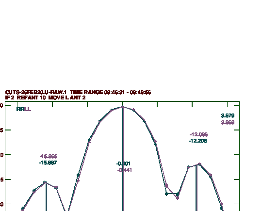
An example of plotting one short raster at 4.8 GHz has inputs

Now, to continue the holography analysis, we write out the data in appropriate text files. An example, would be

This will write a file named MYAREA:HOLO00-08RR01 and one named MYAREA:HOLO00-08LL01. Note that we did not specify the one IF to be used, so IF number one was what we got.

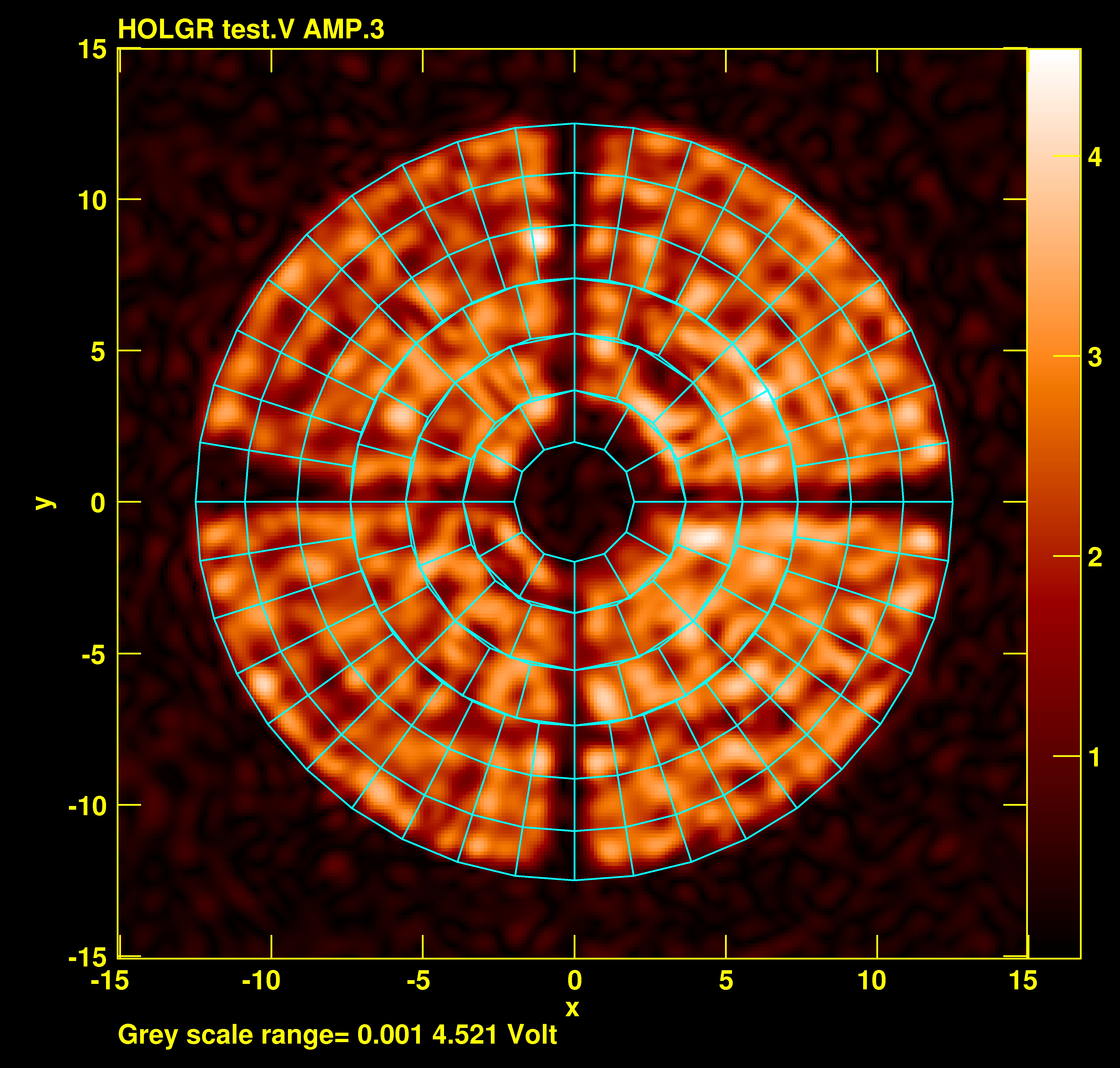
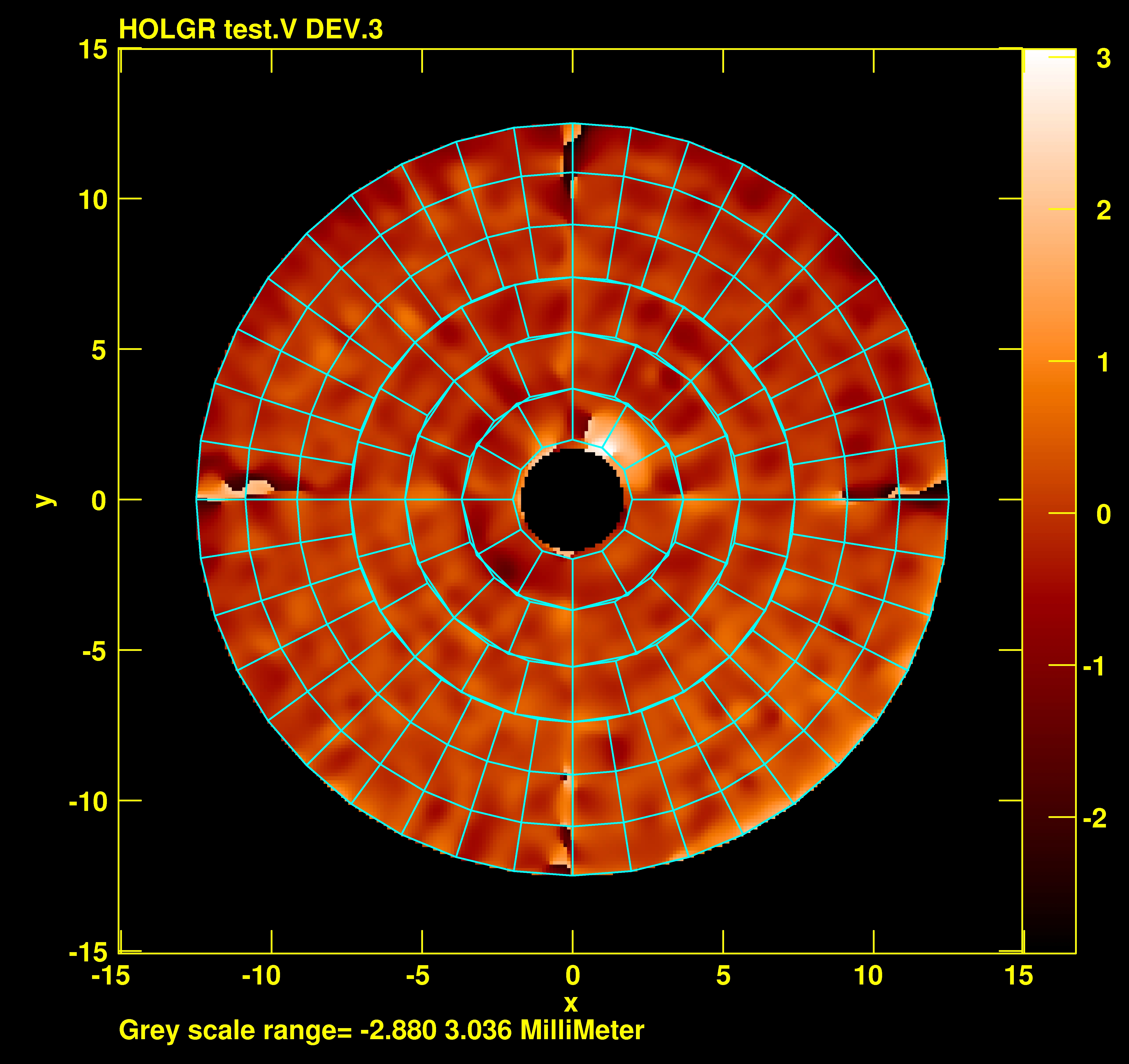
HOLOG reads the visibility data from the text file produced by UVHOL. It can read either amplitude and phase or real and imaginary (APARM(7) in UVHOL). It then Fourier transforms the data to produce the grading in the aperture plane of the antenna. Images of the re-gridded observed amplitude and phase (A_AMP, A_PHA), of the weights in the re-gridding (WGT), of the derived amplitude and phase of the illumination in the antenna aperture (V_AMP, V_PHA), of the amplitude and phase of the point-spread function (P_AMP, P_PHA), of the phase corrections removed by the focus model (MODEL), of the surface deviations of the antenna (V_DEV) in meters, and of the interpolated antenna power pattern (A_PWR) may be produced under control of adverb DPARM. Task PANEL requires V_AMP (DPARM(4)) for the mask and V_DEV (DPARM(9) for the deviations. An example of the images produced by HOLOG is shown in Figure V.3.

Many of the control adverbs must be set to appropriate values. A sample set of inputs is

BPARM specifies the required image size in meters, the image size in pixels, minimum and maximum antenna scan angle, amplitude scaling factor, Fourier transform control (-2 says use DFT with VLA sign convention), minimum and maximum coordinate used in correcting for pointing, focus, and feed offset (negative says in the radial coordinate), a control parameter (100 inhibits local phase ambiguity correction in the V_PHA plane, 8000 turns on finding the Cassegrain offset), and type of data (-1 for VLA). The image size in meters is a function of frequency. To avoid this, CELLSIZE may be set to override BPARM(1) when analyzing multiple frequencies. CPARM all zero says to use the default spheroidal function in gridding on both L and M axes; highly recommended, but not relevant when using DFT imaging. Note that HOLOG can also generate images from a feed model using VPARM.

In 31DEC23, an experimental task HOCLN was written to do a Clean operation on the images produced by HOLOG. Normally, data sampling in holography is essentially on a regular grid at or less than the critical sampling. As a result, this complex Clean operation usually is of little value.

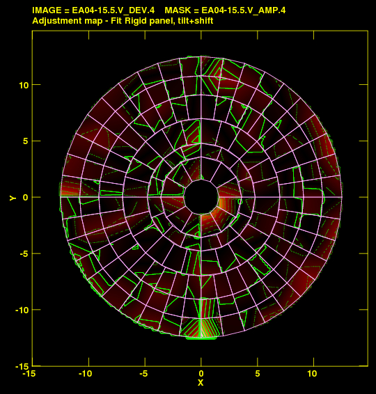
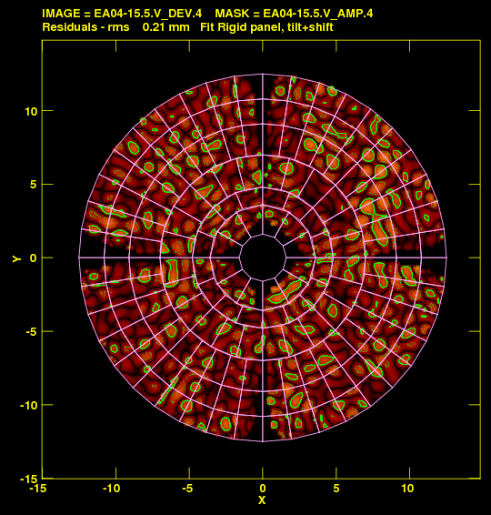
The last task in the process of measuring corrections to the antenna surface is PANEL

The corrections are determined by fitting all samples in each panel to a model of a rigid panel with only shift or with tilt and shift or a flexible panel. There are a large number of samples in each panel, so in 31DEC23, an option to omit samples near the edges of panels was added. This APARM(6) option allows the user to suppress effects spilling over from adjacent panels. Example plots of the panel adjustments and residual are shown in Figure V.4. Adding 8 to DOPLOT produces an image of the dish with all panels marked to show the corner definitions which rotate around the dish.

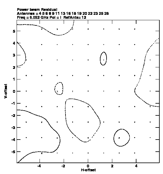
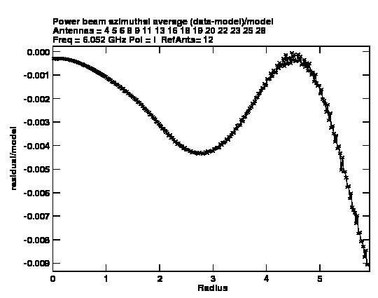
With appropriate holography data, the output of UVHOL may also be used to fit an analytic function to the primary beam. The task that does this is called PBEAM and it fits a polynomial function and makes contour plots of the input data, the fit model, the residual, and IRING-like plots comparing data and model in two colors, and then IRING-like plots of the residual image and residual image divided by the model. Plots against radius of the smooth model with the data points and of the residuals may also be generated.

Sample inputs could contain

Sample plots are shown in Figure V.5.